Chance nodes and expectimax, why pruning stops paying, depth-limited expectimax, where the probabilities come from, what goes wrong when your model of the opponent is wrong, expectiminimax on mixed layers, and Monte Carlo tree search (MCTS) with its selection rule UCB1 (upper confidence bound, version 1) and the full algorithm UCT (upper confidence bounds applied to trees).
Printed copy: all task answers below are revealed. On screen they are hidden behind a click, which is how you should use them first.
The August 2023 sample paper contains no question from this Part. The reference notes state this explicitly: the sample paper has no question from Parts 1, 3, 8 or 14. So unlike Part 5 or Part 7, you cannot look up "how they asked it last time" for expectimax or Monte Carlo tree search. Two facts decide how to read that:
we try to make the exam balanced in terms of topics... you will see that it's uh very well balanced in terms of topics.(Lecturer, T9), hedged in the same breath by the admission that they cannot ask you everything. Balance is his aspiration, not an observed property of the 2023 paper.
Practical reading: prepare Part 8 as if it will be asked, and prepare it in the exercise-session format, since that is the format in which this material comes with published solutions. The session itself says that trees of this kind have been exam questions in the past (quoted in section 19), so the absence of a Part 8 question in one sample paper is not evidence that the material is safe to skip.
Part 7 gave you a game tree with two kinds of internal node: MAX takes the maximum of its children, MIN takes the minimum. This Part replaces the MIN layer, in some or all of its occurrences, with a third kind of node:
Deck p.5 states the substitution in the lecturer's phrasing: chance nodes "are like min nodes but the outcome is uncertain", so you "calculate their expected utilities", that is, "take weighted average (expectation) of children". Everything else in the algorithm is untouched. That single substitution is what generates the rest of the Part: pruning stops working (section 5), the depth limit behaves differently (section 6), you now need a probability model (sections 7 to 9), and getting that model wrong has a specific and measurable cost (sections 10 and 11).
Deck p.5 also lists the three reasons the outcome of an action may be unknown, and it is worth keeping all three in mind because only the first one looks like a game:
The third one is not about games at all, and it is the bridge to Part 9: the same slide says that these uncertain-result problems will later be formalised as Markov decision processes (MDPs).
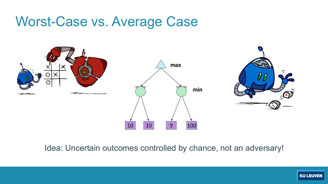
The two middle nodes are drawn as green circles with a red MIN triangle still showing underneath, because this slide is a flattened animation of the substitution itself. Read the tree twice: once with the middle layer as MIN, once with the middle layer as chance nodes with uniform probabilities. Give the root value each time and say which child the root chooses each time.
As MIN: left = min(10, 10) = 10, right = min(9, 100) = 9, root = max(10, 9) = 10, and the root goes left.
As chance, uniform: left = (10 + 10)/2 = 10, right = (9 + 100)/2 = 54.5, root = max(10, 54.5) = 54.5, and the root goes right.
Why it matters: the same four numbers produce opposite decisions. The 100 is invisible to MIN, because an adversary would never hand it to you, and dominant under an expectation, because chance sometimes will. This is why the answer to "which algorithm" is never cosmetic.
Constructed, in the sample paper's format. Built on the verified p.4 tree; the 2023 sample paper has no Part 8 question
The tree on p.4 has four leaves: 10 and 10 under the left middle node, 9 and 100 under the right one. Reading that middle layer as chance nodes with uniform probabilities instead of as MIN nodes changes the move the root selects.
Expectimax search computes, in the deck's words on p.5, "the average score under optimal play". Optimal play refers to the MAX agent, who is still assumed to play the best move available. Average refers to everything outside the agent's control.
The pseudocode on p.8 is deliberately written as a dispatcher plus two workers, exactly parallel to the minimax code from Part 7:
Two details in that code are worth naming, because they are what a fill-in question would target. First, the initialisation differs: -∞ for a maximum, 0 for a sum. Second, the probability is attached to the arc, not to the child, which is why an unlabelled arc in an exam figure is a missing piece of data rather than a detail you may ignore.
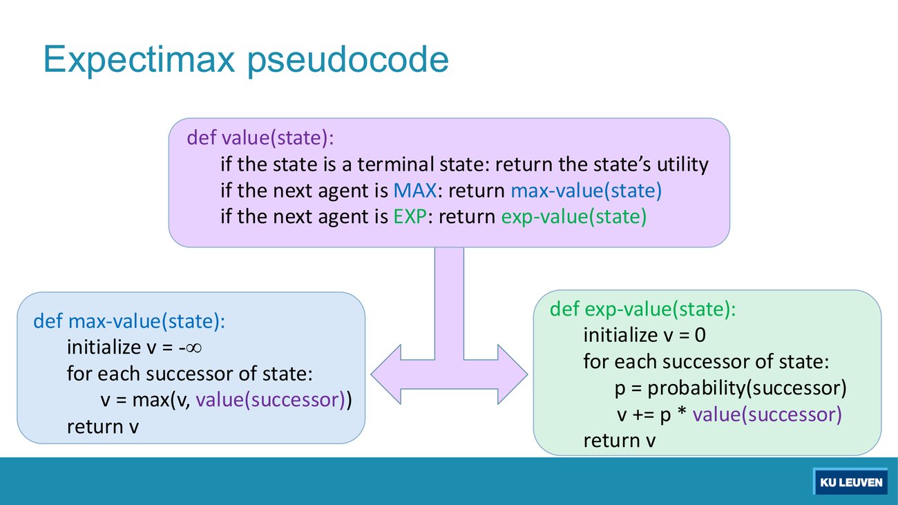
A student "optimises" exp-value by initialising v = -∞ to match max-value, and separately decides that when a chance node has a single successor the loop can be skipped and the child's value returned directly. Which change is fatal, which is harmless, and why?
The initialisation is fatal. v is an accumulator for a sum, so it must start at the additive identity, 0. Starting at -∞ makes every chance node evaluate to -∞, because -∞ + p·value is still -∞.
The single-successor shortcut is harmless, but only because a distribution over one outcome must give it probability 1, by the law that probabilities over all possible outcomes sum to one (p.14). So v = 1 · value(child). If the single arc were labelled with anything other than 1, the tree itself would be malformed.
Constructed, in the sample paper's format. Tests the p.8 pseudocode, in the style of the 2023 fill-in block (questions 2.1 and 2.2)
In the exp-value routine printed on p.8, what is v initialised to before the loop over successors?
Deck p.9 repeats the exp-value code beside a single chance node with three children and prints the arithmetic in full: the arcs carry 1/2, 1/3 and 1/6, the leaves are 8, 24 and −12, and the printed result is
v = (1/2)(8) + (1/3)(24) + (1/6)(−12) = 4 + 8 − 2 = 10
Verified. Note what the number is not: it is not any child's value, it is not between the two most likely children, and it is larger than two of the three leaves. An expectation is not a summary statistic you can eyeball, it is a computation.
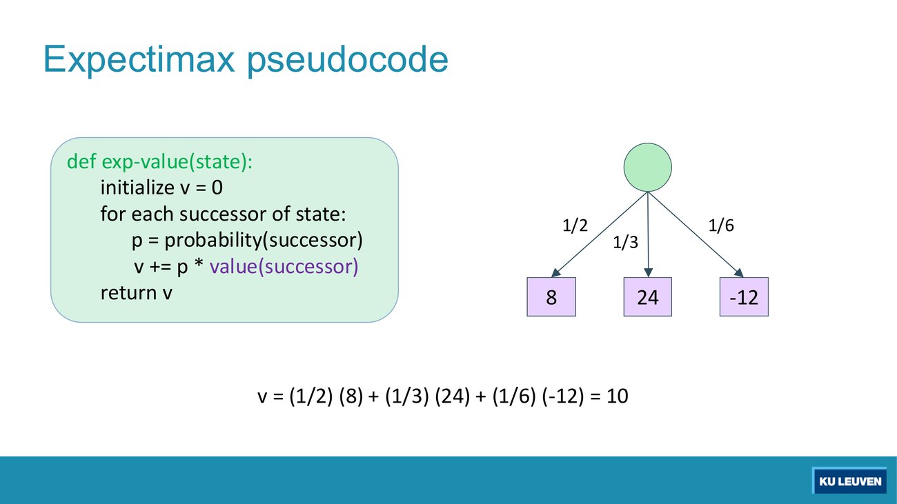
Keep the leaves 8, 24 and −12 and replace the printed weights by a uniform distribution over the three children. Compute the new value, then say in one sentence what the change of weights did and why.
Uniform means p = 1/3 each, so v = (8 + 24 − 12)/3 = 20/3 = 6.67 (exactly 20/3), down from 10.
Why: the printed distribution puts 1/3 of the weight on the best outcome (24) and only 1/6 on the worst (−12). Flattening to uniform moves weight from the good outcome onto the bad one. The tree structure did not change at all; only the model of the world did. That is the whole content of sections 7 to 9.
Constructed, in the sample paper's format. A chance-node value computation; arithmetic executed in Python
Keep the three leaves of p.9, that is 8, 24 and −12, and change the arcs to carry 0.25, 0.25 and 0.5 in that order. What is the value of the chance node?
Deck p.10 is the one full expectimax tree in the deck: a MAX root, three chance nodes, and nine leaves in three groups, 3 12 9 on the left, 2 4 6 in the middle, 15 6 0 on the right. The arcs carry no printed probabilities, checked both on the rendered slide and in the extracted text layer of that page, so the intended reading is the uniform one, 1/3 per child, which is also the reading that makes the numbers come out whole.
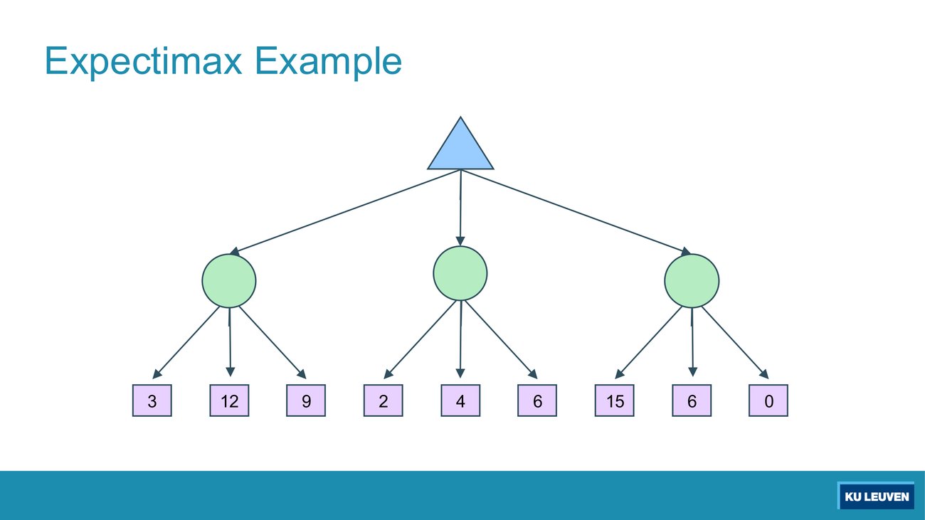
Fill in the three chance values and the root, with 1/3 on every arc. Then, for the same tree, write down what a student gets if the chance layer is mistakenly treated as a MIN layer, and what they get if it is mistakenly treated as a MAX layer. Which of the three answers picks which move?
| Reading of the middle layer | Left | Middle | Right | Root | Move chosen |
|---|---|---|---|---|---|
| Chance, uniform (correct) | 8 | 4 | 7 | 8 | left |
| MIN (the classic mistake) | 3 | 2 | 0 | 3 | left |
| MAX (the other slip) | 12 | 6 | 15 | 15 | right |
Arithmetic: (3 + 12 + 9)/3 = 8, (2 + 4 + 6)/3 = 4, (15 + 6 + 0)/3 = 7, root = max(8, 4, 7) = 8. All three verified.
The classic mistake is applying min at a chance node, and it is seductive here because it happens to choose the same move as the correct reading. It gets you the wrong number, and on a tree where the right branch contained one very large leaf it would also get you the wrong move. Never let a chance node take an extremum. Also note the reporting habit that gets marks: if the arcs are unlabelled, write "assuming a uniform distribution" beside your answer rather than silently assuming it.
Constructed, in the sample paper's format. Built on the verified p.10 trace table
On the p.10 tree (leaf groups 3 12 9, then 2 4 6, then 15 6 0, with uniform arcs) a student mistakenly treats the chance layer as a MIN layer. That mistake changes the move the root selects.
Deck p.11 asks the question and answers it visually: a MAX root, a left chance node whose three children 3, 12 and 9 are known, and a right chance node whose first child is 2 while the other two arcs trail off into dashes. Alpha-beta pruning worked because a MIN node's value can only go down as more children arrive, so once it drops below a MAX ancestor's alpha you may stop. A chance node has no such one-way behaviour: a partial weighted sum can still move in either direction, and by an unbounded amount, unless you know a bound on the leaf values.
we will not consider pruning in this case... the pruning is very limited.(Lecturer, T7), spoken over p.11. In the lecture he adds that bounds on chance nodes could in principle be defined but come out very loose, so the efficiency gain does not repay the complication. This is a licensed scope limit: expectimax pruning is out of scope for this course. Do not write an alpha-beta trace on an expectimax tree, and if a question asks whether pruning applies, the expected answer is that it is possible in principle only under bounded utilities and is not considered here.
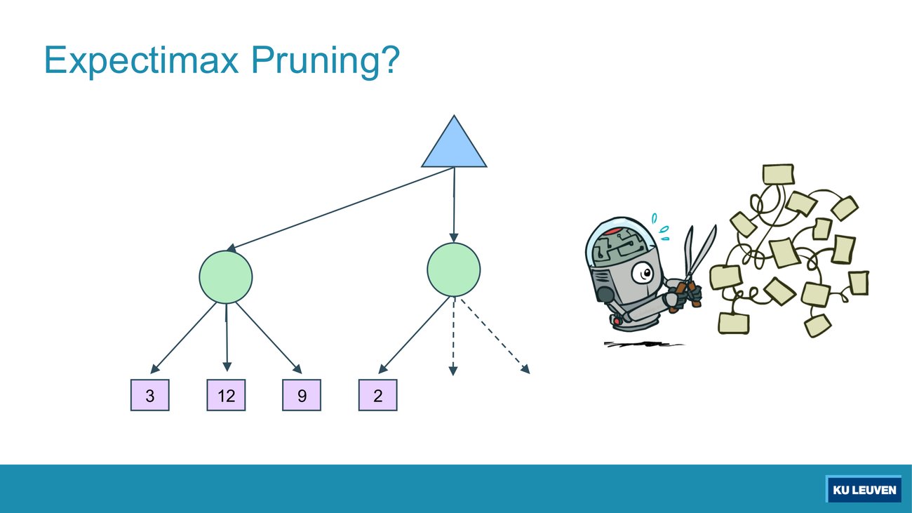
The left chance node evaluates to 8. The right one has seen only its first child, 2, with two children still unexplored, and all three arcs carry 1/3. (a) Why can you not prune the rest of the right subtree? (b) Suppose you are additionally told that the two unexplored leaves lie in [0, U]. For which values of U does the right subtree become prunable? (c) The leaves already visible on this slide run as high as 12. If the unexplored leaves can be as large as the ones you have already seen, does anything prune?
(a) The MIN monotonicity argument is gone. A partial sum at a chance node is not an upper or lower bound on the final value, because the remaining children can pull it either way. With unbounded utilities the right node's value could still turn out to be arbitrarily large, so nothing can be excluded.
(b) With the two unexplored leaves in [0, U] the right node is at most (2 + U + U)/3. Pruning is safe when that ceiling cannot beat the incumbent 8, that is (2 + 2U)/3 ≤ 8, so U ≤ 11. Checks: U = 9 gives a ceiling of 20/3 = 6.67, prunable; U = 10 gives 22/3 = 7.33, prunable; U = 15 gives 32/3 = 10.67, not prunable. All verified.
(c) No. The visible leaves reach 12, so the honest bound to assume here is U = 12, giving a ceiling of (2 + 12 + 12)/3 = 26/3 = 8.67, which is above 8. Nothing prunes on this tree. Note also that the bound has to be stated for the unexplored leaves only: bounding every leaf by U would force U ≥ 12 at once, since 12 is printed on the slide, and then the ceiling can never fall below 8.67.
That is exactly the lecturer's point that bounds "will be very loose": you need a tight, known range on the utilities before anything gets cut, the range you can actually justify from a real game is usually the one that cuts nothing, and this is why the course does not consider expectimax pruning at all.
Deck p.12 keeps the construction from Part 7 and changes only the node types: a MAX root, then a layer of chance nodes for one ghost, then another layer of chance nodes for a second ghost, then a cut-off where an evaluation function returns numbers such as 400 and 300. The callout on the slide names what those numbers are: an "Estimate of true expectimax value (which would require a lot of work to compute)". Below the cut, the deeper values 492 and 362 show what the exact computation would have produced.
Two things change relative to minimax. First, the estimate at the cut is now standing in for a weighted sum rather than for an extremum, so an evaluation function that is merely ordinally correct (ranks states properly) is no longer enough: the magnitudes get multiplied by probabilities and summed, so a monotone rescaling of your evaluation function can change the decision. That first point is a consequence of the arithmetic rather than a printed slide claim, but it follows directly from p.8. Second, as p.28 notes for backgammon, the probability of reaching a given deep node shrinks as depth grows, so cutting depth costs less than it does in a deterministic game.
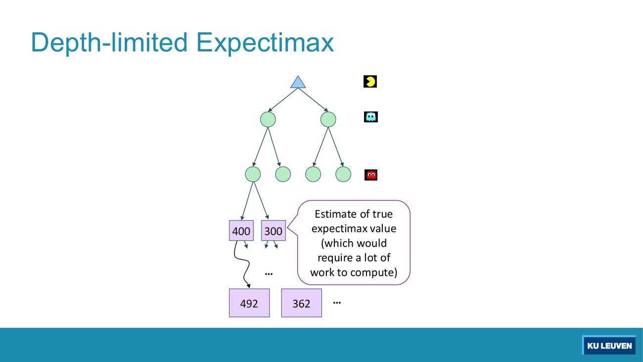
Read the ply structure off the icons on the right of the slide, then answer: how many agents move between the root and the cut-off, what kind of node is each layer, and what exactly is the object that the evaluation function is estimating at 400 and 300?
Three agents appear: Pacman at the root (MAX), then ghost one, then ghost two. So the tree is MAX, chance, chance, and the cut-off sits below the second chance layer. In a two-ghost world one full round of the game is three moves, so a stated "depth" is ambiguous unless you say whether it counts agent moves or full rounds. The drawn tree is exactly one round.
The evaluation function at 400 and 300 is estimating the true expectimax value of that state, that is, the number you would get by expanding the whole subtree and doing every weighted sum. It is not estimating "how good the board looks" in any other sense, and it is not a utility: real utilities only exist at terminal states.
the real solution is not so much increasing the depth... but rather finding an evaluation function that really does account for everything that is genuinely important.(Exercise session, T8). The games exercise session is run by the teaching assistant named on the exercise deck, so these asides carry a different attribution from the lecture asides above. He is explaining why depth-limited Pacman sometimes freezes in place: with a limited horizon, stopping and moving north can receive identical scores, so the agent has no reason to move, and the score bleeds away one point per step. His diagnosis is the exam-relevant part: this is an evaluation-function problem, not an algorithm problem. Deepening the search postpones the pathology instead of removing it, because you can always build a position where nothing within the horizon changes the score.
Deck p.14 is a deliberate one-slide refresher. A random variable represents an event whose outcome is unknown; a probability distribution is an assignment of weights to outcomes. The worked case is traffic, T in {none, light, heavy}, with P(T = none) = 0.25, P(T = light) = 0.50 and P(T = heavy) = 0.25. Two laws are printed: probabilities are always non-negative, and probabilities over all possible outcomes sum to one. The slide then shows that evidence changes a distribution: P(T = heavy) = 0.25 becomes P(T = heavy | Hour = 8am) = 0.60.
which we'll also not further discuss uh here.(Lecturer, T7), said of Bayesian networks while showing the conditional-probability line on p.14. Bayesian networks are named in this course and never developed. This is a licensed scope limit: you are expected to know that updating a distribution on evidence is possible and is what such models do, and you are not expected to compute with one.
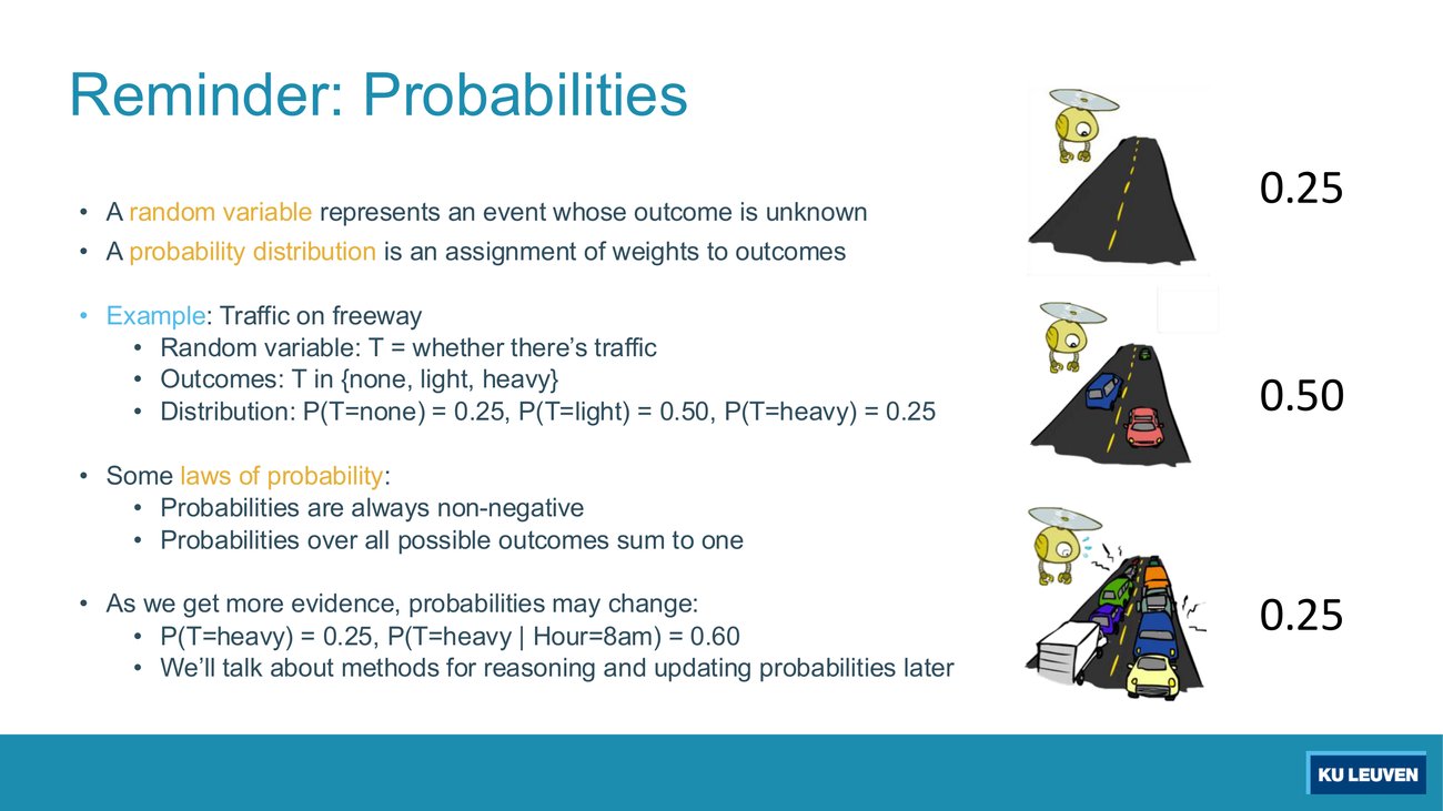
Given the evidence Hour = 8am, the slide states P(T = heavy | 8am) = 0.60. Nothing is printed for the other two outcomes. What can you say about them, exactly, and what can you not say?
What you can say: P(none | 8am) + P(light | 8am) = 1 − 0.60 = 0.40, and both are non-negative. That is forced by the two printed laws.
What you cannot say: how the 0.40 splits. The prior split was 0.25 to 0.50, that is one third to two thirds, but conditioning on evidence is not required to preserve the ratio of the remaining outcomes. Any split summing to 0.40 is consistent with the slide.
This distinction is exactly what a chance node needs from you in an exercise: the missing weight on the last arc is determined, the values behind it are not.
Deck p.15 defines the object the whole Part is built on: the expected value of a function of a random variable is the average, weighted by the probability distribution over outcomes. The example is the trip to the airport, with times 20, 30 and 60 minutes carrying probabilities 0.25, 0.50 and 0.25, and the printed answer 35 minutes.
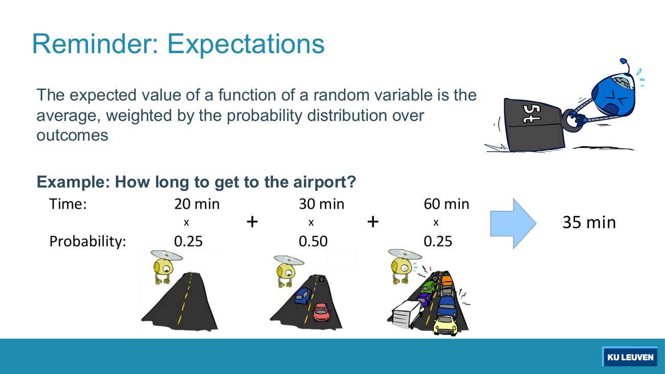
Verify the printed 35. Then recompute with the distribution shifted to 0.10, 0.50, 0.40 over the same times, and say which of the two ingredients, the values or the weights, moved the answer.
0.25(20) + 0.50(30) + 0.25(60) = 5 + 15 + 15 = 35, as printed.
0.10(20) + 0.50(30) + 0.40(60) = 2 + 15 + 24 = 41. Both verified.
Only the weights moved. The set of possible outcomes is identical. That is the sense in which a chance node encodes a model: same tree, same leaves, different answer, and no way for the algorithm to detect that your weights are wrong.
Constructed, in the sample paper's format. Tests the two probability laws printed on p.14
The prior is P(T = none) = 0.25, P(T = light) = 0.50, P(T = heavy) = 0.25, and you are told that P(T = heavy | Hour = 8am) = 0.60. What is P(T = light | Hour = 8am)?
Deck p.16 is the honest slide of the Part. In expectimax search we have a probabilistic model of how the opponent or the environment will behave in any state. The model could be a simple uniform distribution (roll a die), or it could be sophisticated and require a great deal of computation. There is a chance node for any outcome out of our control, opponent or environment, and the slide warns that the model might say that adversarial actions are likely. The last line is the working assumption of the whole Part: for now, assume each chance node magically comes along with probabilities that specify the distribution over its outcomes.
The slide's side note is the sentence most worth carrying into an exam: having a probabilistic belief about another agent's action does not mean that the agent is flipping any coins. The randomness is in your knowledge, not necessarily in the world.
Deck p.17 poses a concrete question. Your opponent is actually running a depth-2 minimax, using the result 80% of the time and moving randomly otherwise. What tree search should you use? The slide answers "Expectimax", and prints 0.1 and 0.9 on the two arcs under a chance node. It then lists the cost: to figure out each chance node's probabilities you have to run a simulation of your opponent, which gets very slow very quickly, and worse if you have to simulate your opponent simulating you. Minimax has the nice property that it all collapses into one game tree.
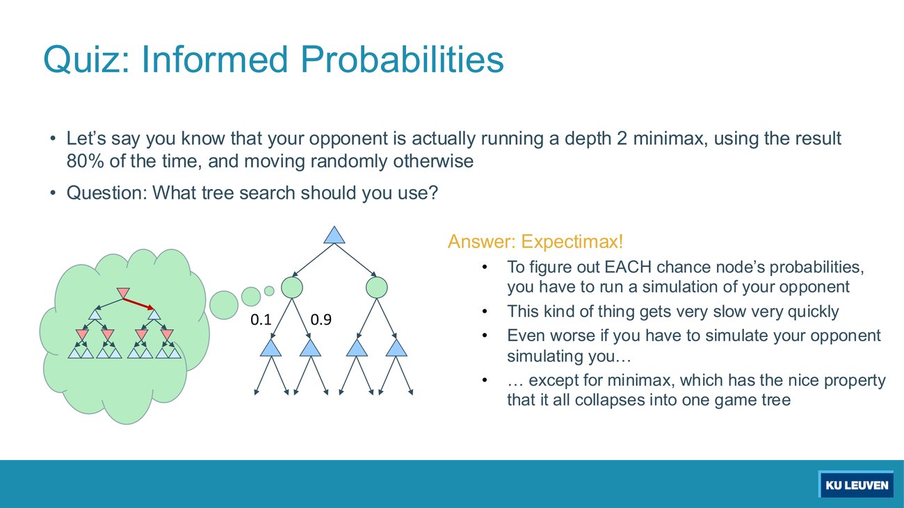
The chance node in the picture has exactly two children. Derive 0.9 and 0.1 from the 80% statement. Then say which of the two children carries the 0.9 and why the answer would change if the node had three children.
Let m be the move that depth-2 minimax recommends and o the other move. The opponent plays m with probability 0.8 outright, and with the remaining 0.2 moves uniformly at random over the two available moves, so each gets an extra 0.2 × 0.5 = 0.1.
P(m) = 0.8 + 0.1 = 0.9, P(o) = 0.1. Verified. The 0.9 sits on the minimax-recommended child.
With three children: P(m) = 0.8 + 0.2/3 = 0.867 and each other child gets 0.2/3 = 0.067. So the printed 0.9 and 0.1 are not a rule to memorise; they are the output of a branching-factor-dependent computation, and you must first run the opponent's minimax to know which child is m at all. That is the meta-reasoning cost the slide is complaining about.
Deck p.19 names the two ways a model can be wrong, and gives each a one-line definition:
These are not symmetric in their consequences, and the next two slides measure the asymmetry. Optimism gets you killed. Pessimism costs you time and score but usually still wins.
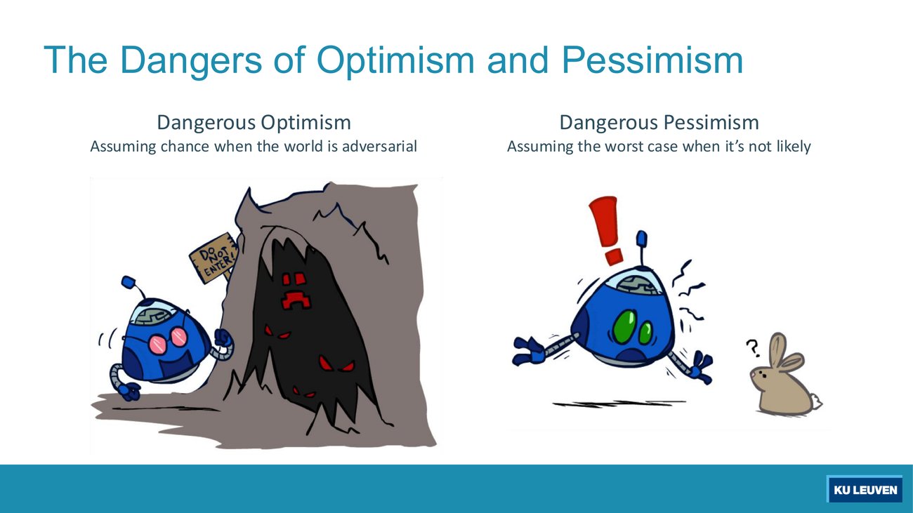
For each of the two pictures, say which algorithm the agent is running and which assumption it is making, then state which chance-node computation the agent should have used instead.
Cave (dangerous optimism): the agent is running expectimax, averaging over the monster's possible responses, in a world where the monster actually minimises. It should have used min at that layer, that is, minimax.
Rabbit (dangerous pessimism): the agent is running minimax, treating a harmless random entity as an adversary. It should have used a weighted sum at that layer, that is, expectimax.
The general statement: the error is not in the search algorithm, it is in the node type you assigned to the other agent's layer. Both agents searched correctly, over the wrong tree.
Deck pp.20 and 21 are the same slide twice, once with the four result cells empty and once filled in. The lecture spends roughly ten minutes on it, most of that on the two off-diagonal cells, and the four demo slides that follow (pp.22 to 25) play out one cell each. The experimental setup is printed on both pages and is part of the answer, so read it before the numbers:
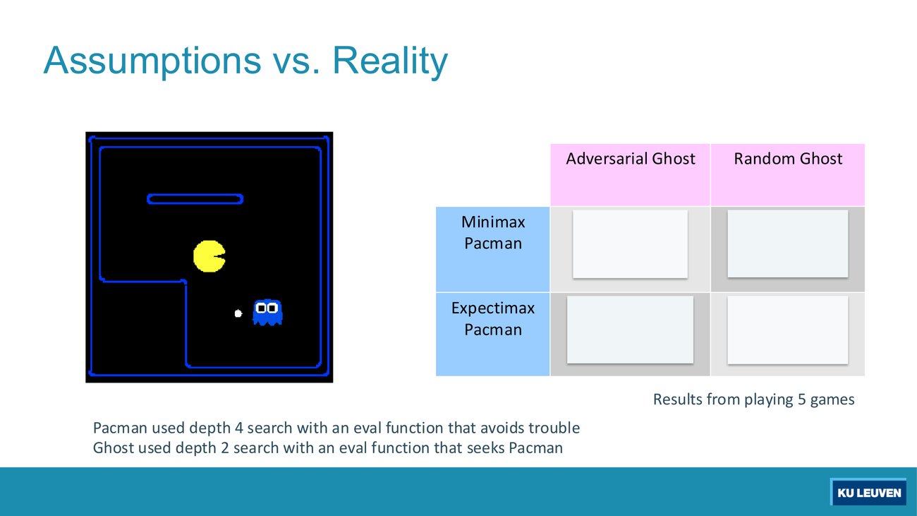
The four cells are still empty in this figure. For each of the four combinations, predict whether Pacman wins all five games, wins about one, or something in between, and rank the four average scores from best to worst. Commit to an answer before opening the next figure.
Wins: both diagonal cells 5/5; minimax against the random ghost also 5/5; expectimax against the adversarial ghost about 1/5.
Score ranking, best to worst: expectimax vs random (503), minimax vs random (493), minimax vs adversarial (483), expectimax vs adversarial (−303).
The reasoning that gets you there without the numbers: a wrong assumption in the safe direction costs efficiency, a wrong assumption in the unsafe direction costs the game. So three cells win and one collapses, and the collapse is the cell where the model is optimistic.
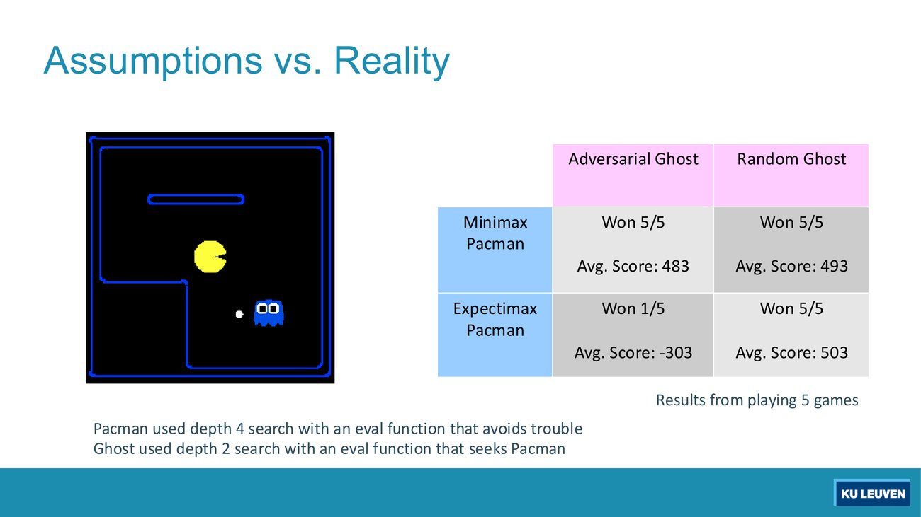
The expectimax and adversarial cell prints "Won 1/5, Avg. Score: −303", while the expectimax and random cell prints "Won 5/5, Avg. Score: 503". Assuming a win in the losing cell scores about the same as a win in the winning cell, what does a loss score, roughly? What does that tell you about the shape of the utility function in this Pacman world?
Let a win be worth about +503 and a loss L. Then (503 + 4L)/5 = −303, so L ≈ −504.5. Verified: (503 + 4(−504.5))/5 = −303.0 exactly.
What it tells you: the outcome term dominates everything else by two orders of magnitude over the per-step cost. Winning and losing are roughly ±500, while an extra step costs about 1. That is why the safe strategy is cheap insurance: hundreds of wasted steps still cost less than one avoidable death. It is also the reason the two winning columns differ by only 10 points (493 vs 503, and 483 vs 493).
Mark this as an inference from the printed numbers rather than a printed fact: no scoring rule appears anywhere on pp.20 and 21, checked against the extracted text of both pages, which carry only the two win/score lines per cell and the three setup lines.
Why does this cell win, and why is its score lower than the cell directly to its right?
It wins because the assumption matches reality: Pacman assumes a rational opponent and faces one, so his plan is valid against the moves that actually occur. The lecture calls this the perfect alignment on the diagonal.
Its score is lower than 493 because a genuinely hostile ghost forces detours: Pacman must play the safe line, feint away from the pellet, and only then collect it. Every extra step costs score. The win is never in doubt; the efficiency is.
This is dangerous pessimism, yet it wins all five games. Explain why pessimism is not punished here, and state the one condition under which this cell would still be a bad choice.
Minimax computes a value under the worst case. The random ghost's actual behaviour is a distribution over moves, and the worst case is one of the outcomes in that distribution. So a plan that survives the worst case survives everything the random ghost can do. Over-preparing cannot lose you a game; it can only waste moves.
In the lecture's demo the wasted moves are visible: Pacman runs from a ghost that is not chasing him, the running score dips well below zero, and he still finishes ahead because eating the pellet is worth far more than the steps it cost (the roughly ±500 versus 1 asymmetry of the previous task).
The condition under which it is a bad choice: when the game rewards speed enough that the wasted steps outweigh the safety, or when a game is time-limited. Change the scoring so a step costs 50 rather than 1 and this cell stops winning on points.
This is the only cell that collapses. Say precisely which computation produces the fatal move, in terms of the node values, rather than in terms of "the assumption was wrong".
At the ghost's layer Pacman computes a weighted average over the ghost's moves instead of a minimum. Constructed example: suppose the ghost has k moves and exactly one of them eats Pacman with value about −500 while the others are near 0. The chance node reports roughly −500/k, which for k = 4 is −125, a number Pacman is willing to accept in exchange for a nearby pellet. Minimax at the same node reports −500 and refuses the line.
So the fatal step is that averaging dilutes a catastrophic outcome by the branching factor, while an adversary selects exactly that outcome with probability 1. The larger the ghost's branching factor, the more the danger is diluted and the more confident the mistake becomes.
The single win in five is real, not a rounding artefact: an optimistic agent that takes risks sometimes gets away with it. That is why the cell reports 1/5 rather than 0/5.
This cell has the best score in the table. Is that because expectimax is the better algorithm? Answer with the general rule this table is teaching.
No. It has the best score because its model matches reality and the reality is benign, so it wastes no moves on defence it does not need. Pacman goes more or less straight to the pellet.
The general rule: the algorithm is not good or bad in itself; what is graded is the match between the node type you assign to the other agent's layer and how that agent actually behaves. The diagonal wins on both counts. Off the diagonal, one direction of mismatch costs score and the other costs the game. If you must be wrong, be wrong pessimistically.
The lecturer also flags the sample size: five games. The random ghost cell in particular could produce a loss on another run, since Pacman can be unlucky even when acting rationally.
Constructed, in the sample paper's format. Cell values read off p.21
One cell of the assumptions-versus-reality table prints "Won 1/5, Avg. Score: −303". Which cell is it?
Deck p.27 introduces the third algorithm by drawing it: a MAX root, then a layer of chance nodes, then a layer of MIN nodes, then leaves. The two printed bullets are the whole definition. The environment is an extra "random agent" player that moves after each min or max agent, and each node computes the appropriate combination of its children. The name is expectiminimax, and the example game is backgammon: you roll, then you move, then your opponent rolls, then your opponent moves.
Deck p.28 quantifies the cost. Dice rolls increase the branching factor b: there are 21 possible rolls with 2 dice, and backgammon has roughly 20 legal moves, so the slide writes depth 4 as 20 × (21 × 20)3. Three consequences follow on the same slide: as depth increases the probability of reaching a given search node shrinks, so the usefulness of search is diminished, so limiting depth is less damaging, but pruning is trickier. The historical note is TDGammon, which reached world-champion level with depth-2 search, a very good evaluation function and reinforcement learning, and was the first AI world champion in any game.
Arithmetic note: the deck prints the result of that product as 1.2 × 10⁹. Multiplying the expression exactly as printed gives 20 × 4203 = 1.48 × 10⁹. The slide is making an order-of-magnitude point, so reproduce the construction of the product in an exam, not the digits.
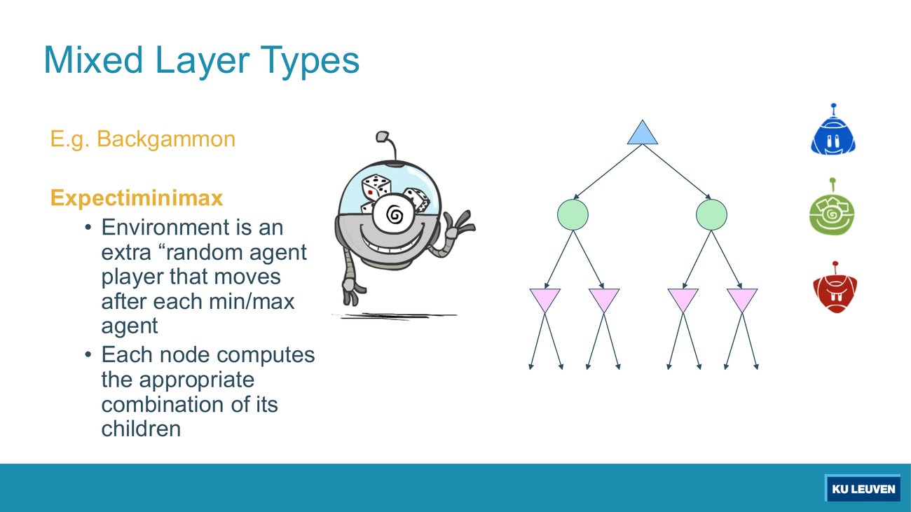
Walk down the drawn tree and label every layer with (a) who acts, (b) which operation the node performs. Then extend the pattern by one more ply and say what comes after the MIN layer. Finally: on a backgammon turn, does the player choose before or after the dice are known, and which node ordering encodes that?
Root: MAX agent, takes a maximum. Layer 2: the environment, takes a probability-weighted sum. Layer 3: MIN agent, takes a minimum. The next ply is another chance layer, because the environment moves after each min or max agent, then MAX again. The repeating unit is MAX, chance, MIN, chance.
The dice are known before the move is chosen: you roll, then you decide. That is why the chance node sits above the player's node in the tree, so that the player's maximisation happens inside each roll outcome, not before it. Reversing the order would model a player who must commit to a move before seeing the roll, which is a different game.
Constructed, in the sample paper's format. Tests the layer ordering printed on p.27
In the expectiminimax model of backgammon on p.27, the player commits to a move before the dice roll for that turn is known.
Deck p.29 puts the three algorithms side by side with a game for each: minimax for tictactoe and chess, expectimax for Tetris and investing, expectiminimax for backgammon and Monopoly. It is the slide that answers "which algorithm" questions, and it is worth memorising as a picture, because Part 9 opens by reusing it unchanged as its second page.
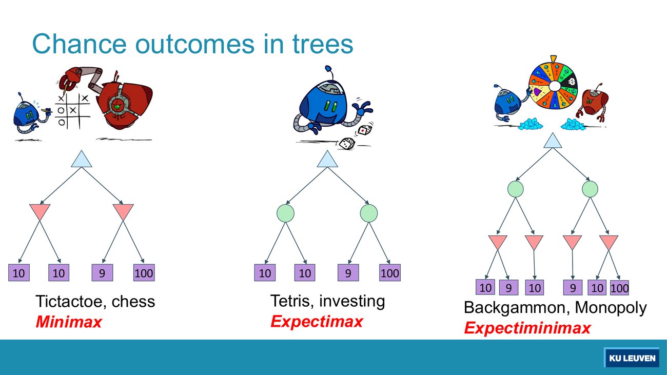
The left and middle trees carry the same four leaves, 10, 10, 9, 100. The right tree has six leaves, grouped 10 9 then 10 then 9 then 10 100 under four MIN nodes, two per chance node. Compute all three root values with uniform probabilities at every chance node, then explain the ordering you get.
| Tree | Intermediate values | Root |
|---|---|---|
| Minimax (left) | min(10, 10) = 10, min(9, 100) = 9 | 10 |
| Expectimax (middle) | (10 + 10)/2 = 10, (9 + 100)/2 = 54.5 | 54.5 |
| Expectiminimax (right) | MIN layer: 9, 10, 9, 10; chance layer: 9.5, 9.5 | 9.5 |
All verified. The ordering is the lesson. Expectimax is the highest because nothing filters the 100 before it is averaged in. Expectiminimax is the lowest because the MIN layer removes the 100 first (min(10, 100) = 10) and only then is an average taken, so the average is over already-pessimised values. Minimax sits between them here.
Classic mistake: averaging first and then minimising, or reading the right-hand tree as if the chance layer sat below the MIN layer. The order of the layers is the model, and swapping it is not a shortcut.
Deck p.31 opens the second half of the Part with the failure it is designed around. Methods based on alpha-beta search assume a fixed horizon, which is "pretty hopeless for Go, with b > 300". Monte Carlo tree search (MCTS) combines two ideas, and the deck states both twice, on p.31 and again in the summary on p.42:
Notice what is missing compared with everything before it. There is no evaluation function, and there is no fixed depth. The value of a position is estimated by playing from it, many times, badly but quickly, and counting how often that ends in a win.
Deck p.32 gives the simplest possible combination: do N rollouts from each child of the root, record the fraction of wins, pick the move that gives the best outcome by this metric. The printed tree shows a blue MAX root with three red children carrying 57/100, 39/100 and 65/100 from left to right.
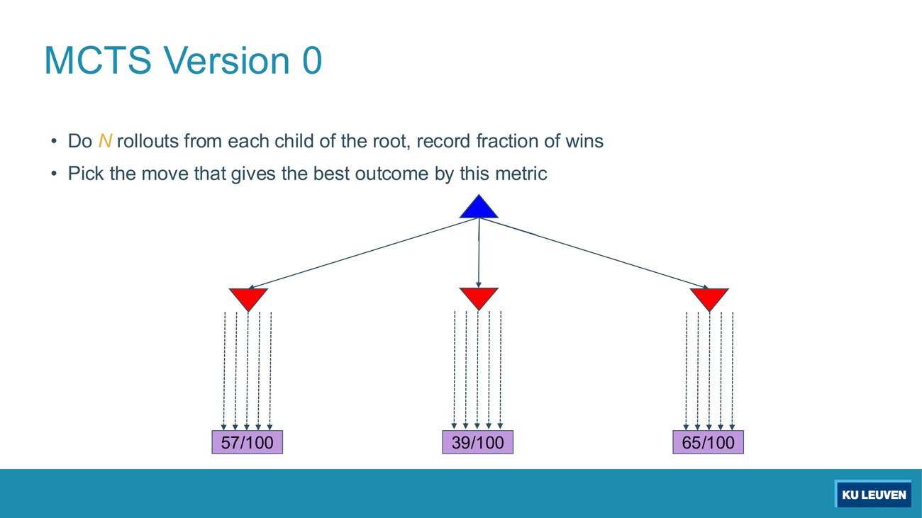
Which move does version 0 select, what is the total rollout budget spent, and what fraction of that budget contributed nothing to the decision that was actually made?
Win rates are 0.57, 0.39 and 0.65, so version 0 selects the right child. The budget is 3 × 100 = 300 rollouts.
The decision is between the right child and its nearest rival, the left child at 0.57. The middle child at 0.39 was never a candidate after the first handful of rollouts, so most of its 100 rollouts bought nothing. Roughly a third of the budget was spent confirming something already obvious, while the close call between 0.57 and 0.65 got no extra evidence.
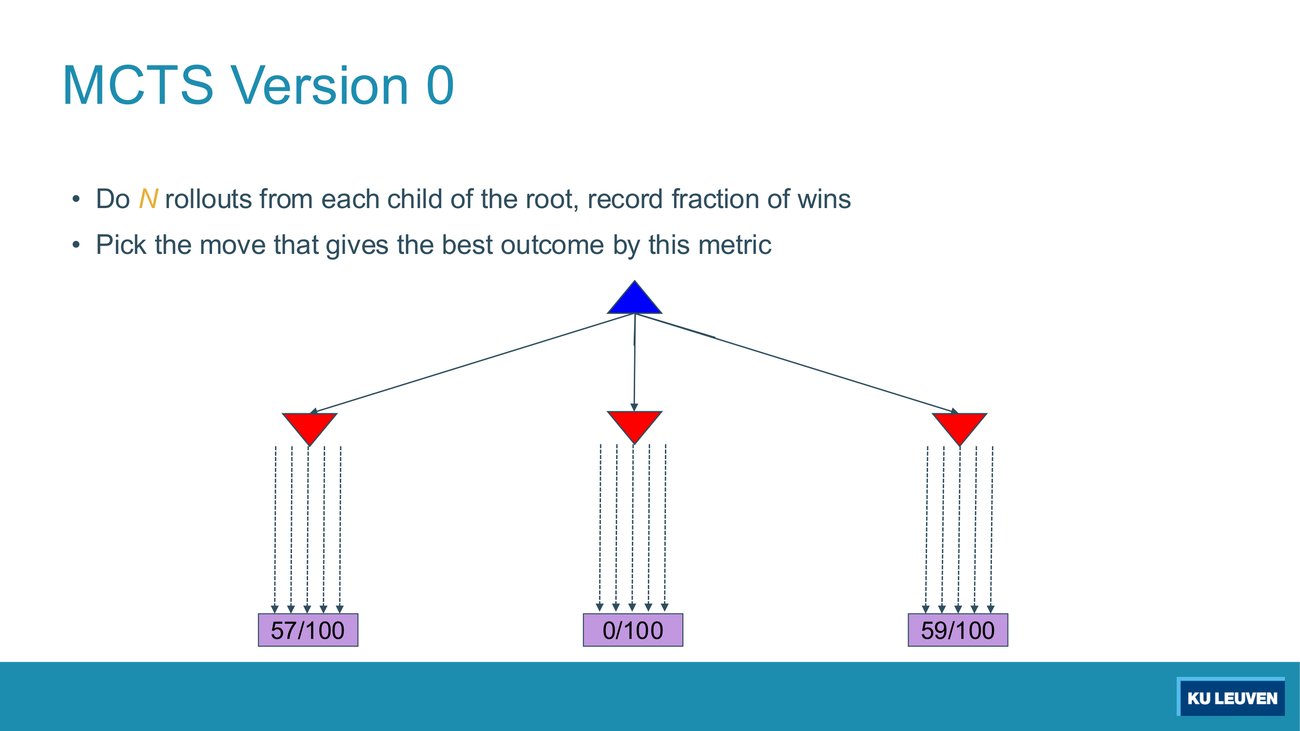
This variant of the same slide shows 57/100, 0/100 and 59/100 from left to right. State the problem in one sentence, then quantify it: after roughly how many rollouts was the middle child's fate already clear, and where should the remaining budget have gone?
The problem: the budget is spread uniformly, so 100 rollouts are spent on a child that loses every single game, while the two children that actually compete, 0.57 and 0.59, are separated by two percentage points and never get the evidence needed to tell them apart.
The lecture puts the point at about 20 rollouts: after roughly 20 straight losses the middle child is clearly hopeless. The remaining 80 should have been split between the left and right children, whose difference is within the noise of 100 samples.
This is the argument for version 0.9: allocate rollouts to more promising nodes.
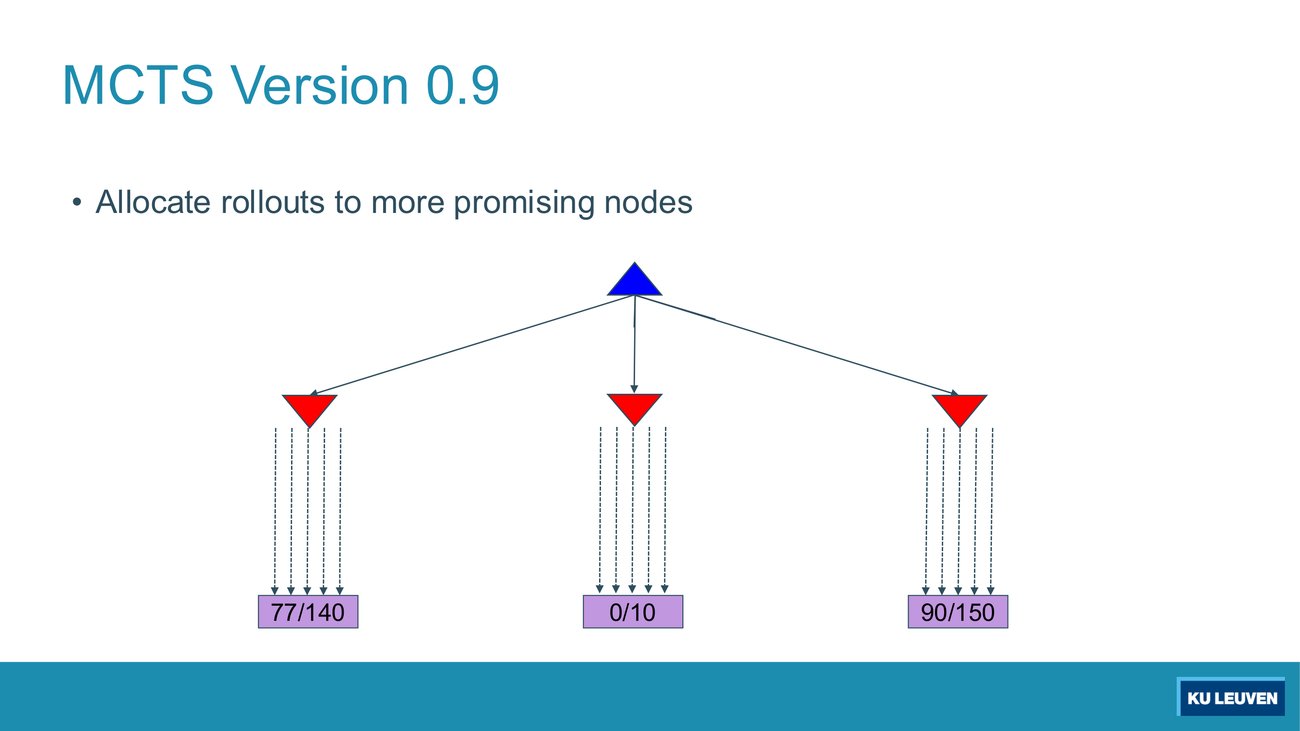
Compute the win rate of each child and the total budget, then compare with p.32's uniform allocation. What did the reallocation buy, in one sentence?
| Child | Record | Win rate |
|---|---|---|
| Left | 77/140 | 0.550 |
| Middle | 0/10 | 0.000 |
| Right | 90/150 | 0.600 |
Budget: 140 + 10 + 150 = 300, exactly the same as the uniform allocation on p.32. All verified.
What it bought: the hopeless child was abandoned after 10 rollouts, and the 90 rollouts saved were spent separating the two real candidates, which now rest on 140 and 150 samples instead of 100 each. Same cost, sharper decision.
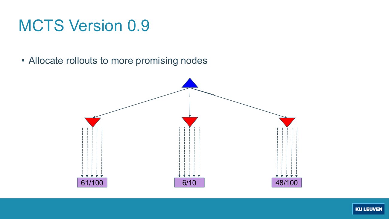
This scenario reads 61/100, 6/10 and 48/100. Version 0.9 sends its next rollouts to the most promising node. Which node is that by win rate, and why is that answer wrong in a way version 0.9 cannot see?
Win rates: 0.61, 0.60, 0.48. By win rate the left child is most promising, by a single percentage point, so version 0.9 keeps feeding rollouts to the left child.
What version 0.9 cannot see: the left estimate rests on 100 samples and the middle estimate on 10. A 0.60 based on 6 wins out of 10 is nearly uninformative; the true value could easily be well above 0.61. Ranking by the point estimate alone treats a well-measured 0.61 and a barely-measured 0.60 as almost equal evidence, when they are not equal evidence at all.
The missing ingredient is a term that rewards uncertainty, which is exactly what version 1.0 adds.
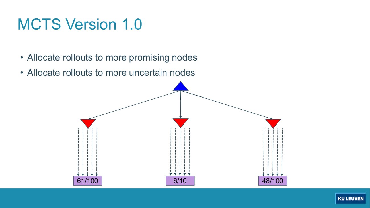
The tree is numerically identical to the previous figure; only the bullet list has grown by one line. Which child does version 1.0 send its next rollouts to, and what quantity would you have to invent to make that choice mechanical rather than verbal?
The middle child (6/10), because it is nearly as promising as the leader and is by far the least explored, so a rollout there changes your beliefs more than a 101st rollout on the left.
To make it mechanical you need a single number per child that adds a bonus for being under-explored to the observed win rate, so that two effects can be traded off in one comparison. That number is UCB1 in the next section: a score of the form (win rate) + C × (an uncertainty term that shrinks as the node is visited and grows as its siblings are visited).
Deck p.37 prints the formula that turns the last two slides into arithmetic. UCB1 stands for upper confidence bound, version 1, and the slide's definitions are:
UCB1(n) = U(n)/N(n) + C × sqrt( log N(Parent(n)) / N(n) )
Read the two terms separately, because that is how every exam question about this formula is built.
it captures relative uncertainty... when you propagate upwards... the siblings basically are going to ever so slightly increase because there's increased uncertainty now.(Exercise session, T8). This is the single most examinable sentence about UCB1, because it is the part students forget. When a rollout goes through one child, the arithmetic touches three groups of nodes: the visited path (both terms change), the siblings of every node on that path (only the exploration term changes, upward), and everyone else (unchanged). The session also notes that real implementations usually recompute these scores on demand rather than storing them, which is why nothing needs to be "written into" the sibling nodes.
The deck prints C as a symbol and never assigns it a number, checked by searching the extracted text of all 44 pages and by reading the p.37 render. The exercise-session solutions do print numeric UCB values, and those numbers pin C down. Their tree has a root with 13 rollouts and children recorded as 3/5, 2/4 and 1/4, with printed scores 1.61, 1.63 and 1.38. Taking C = sqrt(2) and the natural logarithm reproduces all three to two decimals, and it also reproduces every other printed score in that figure (2.27, 1.77, 1.68, 1.67, 1.18, 2.18). The figure carries thirteen printed UCB labels, nine of them distinct; all thirteen were checked.
So: C = sqrt(2) ≈ 1.414 with natural logarithms is the course's working convention, inferred from the exercise solutions rather than stated on a slide. If you compute UCB1 in an exam, write the C you are using next to your answer. That single line protects you if the grader intended a different constant, and it costs nothing.
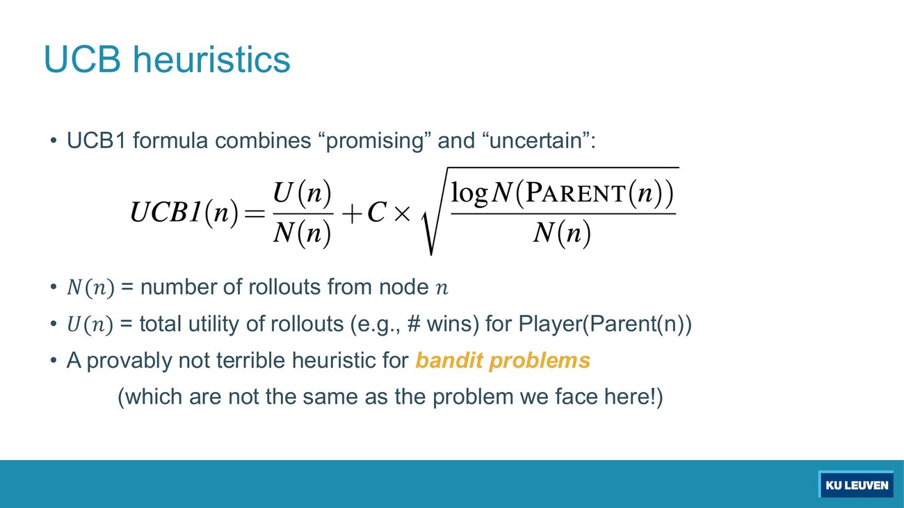
A child has 6 wins out of 10 rollouts and its parent has 100 rollouts. (a) Compute UCB1 with C = sqrt(2) and natural logarithm. (b) A sibling is now visited once, so the parent reaches 101 while this child stays at 10. Does this child's UCB1 rise or fall, and by how much? (c) What would U(n)/N(n) have to be for this child to be tied with a sibling that has 60 wins out of 100 under the same parent?
(a) 6/10 = 0.600, and sqrt(ln 100 / 10) = sqrt(4.60517/10) = sqrt(0.460517) = 0.67861, times sqrt(2) gives 0.95970. UCB1 = 1.5597.
(b) It rises: sqrt(ln 101 / 10) = 0.67935, times sqrt(2) = 0.96074, so UCB1 = 1.5607. The rise is +0.0010, which is the "ever so slightly increase" of the quote above. Small, but the sign is what an exam asks for.
(c) The 100-rollout sibling scores 0.600 + sqrt(2)·sqrt(4.60517/100) = 0.600 + 0.30349 = 0.90349. For the 10-rollout child to tie, its win rate would have to be 0.90349 − 0.95970 = −0.056, which is impossible for a win fraction. So with these visit counts no losing record can pull the sparse child below the well-measured sibling: even 0 wins out of 10 scores 0.9597, still above 0.9035. That is exploration working as designed, and it is why a node with a bad record still gets revisited.
Constructed, in the sample paper's format. Arithmetic executed in Python with C = sqrt(2) and natural logarithms
A node n has 6 wins out of 10 rollouts and its parent has 100 rollouts. A rollout is now sent through one of n's siblings, so the parent reaches 101 while n stays at 10. What happens to UCB1(n)?
the siblings basically are going to ever so slightly increase because there's increased uncertainty now. Tiny in size, but the sign is the whole answer in archetype A16.
Deck p.38 names the complete algorithm, MCTS version 2.0, called UCT (upper confidence bounds applied to trees). The slide gives it as three sub-bullets under "Repeat until out of time", followed by one closing line:
And then, when time runs out: choose the action leading to the child with highest N. Not the highest win rate, and not the highest UCB1. The most-visited child, because under UCT the visit count is the accumulated verdict of every previous selection.
The standard vocabulary for these steps, which is the usual textbook naming rather than slide text, splits the middle bullet in two and calls the four phases select, expand, simulate and back-propagate. Use whichever names you like in an exam, but describe the operations, since only the operations are printed here.
Deck p.39 illustrates one iteration, and it is worth reading carefully because the printed slide is a flattened animation. Two nodes carry two values each, the older one struck through and the newer one beside it:
Reading the struck values as "before" and the plain values as "after" reconstructs the iteration exactly: the middle child was selected, a new child was added under it, the rollout from that child was a win, and the counts were incremented back up the path (0/1 becomes 1/2, and 4/9 becomes 5/10). Nothing off that path changed its counts.
Bookkeeping that has to be right. A node's visit count equals the sum of its children's visit counts plus one, that extra one being the rollout that was run when the node itself was added. Check it on the "after" tree: the root has 7 + 2 + 1 = 10 and is the starting position, so it has no rollout of its own; the left child has 3 + 1 + 2 = 6 from its children plus its own creation rollout, giving 7; the middle child has 1 from its new child plus its own, giving 2. Every count on the slide is consistent. The win counts as drawn add up only if you read every fraction as wins for the player to move at the root (4 + 1 + 0 = 5 at the root, 2 + 0 + 2 = 4 under the left child). The p.37 definition is stricter, U(n) counts utility for Player(Parent(n)), and it is the definition to quote if asked. For selection at the root the two readings agree, which is why the slide can be loose about it.
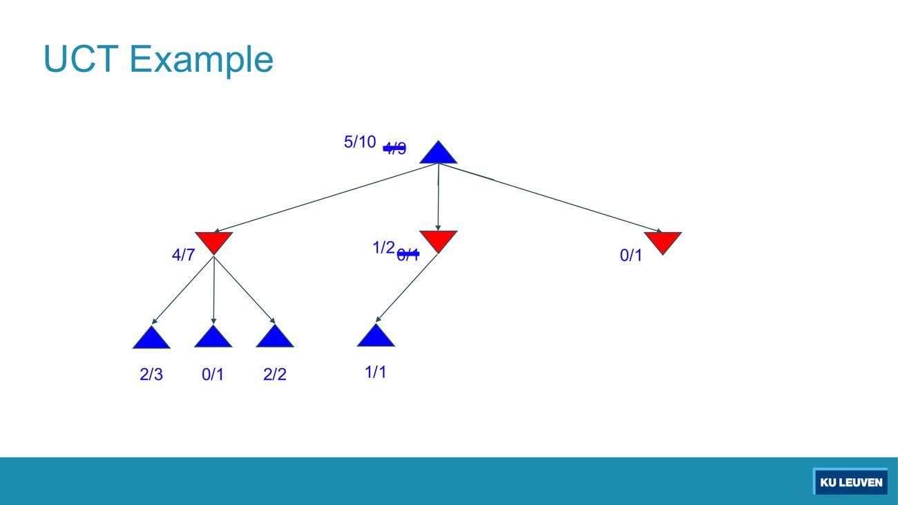
Use C = sqrt(2) and natural logarithms throughout. (a) Reconstruct the "before" tree (root 4/9, children 4/7, 0/1, 0/1) and compute UCB1 for each of the three children. Which child does selection pick, and how is the tie resolved? (b) Now compute UCB1 for the three children of the "after" tree (root 5/10, children 4/7, 1/2, 0/1) and say which child the next iteration will descend into. (c) The middle child just won its rollout. Did its UCB1 go up or down? (d) Which nodes in the tree had their UCB1 changed by this iteration without being visited?
(a) Before, parent N = 9:
| Child | U/N | Exploration | UCB1 |
|---|---|---|---|
| Left, 4/7 | 0.5714 | 0.7923 | 1.3638 |
| Middle, 0/1 | 0.0000 | 2.0963 | 2.0963 |
| Right, 0/1 | 0.0000 | 2.0963 | 2.0963 |
The middle and right children tie exactly, because they have identical records and the same parent. Under the left-to-right tie-break the course states elsewhere (printed in the mixed-belief question of exercise session 5 as "Tie-breaking: choose the left branch", and in the 2023 sample exercise exam), the middle child is taken, which is what the deck's animation shows.
(b) After, parent N = 10:
| Child | U/N | Exploration | UCB1 |
|---|---|---|---|
| Left, 4/7 | 0.5714 | 0.8111 | 1.3825 |
| Middle, 1/2 | 0.5000 | 1.5174 | 2.0174 |
| Right, 0/1 | 0.0000 | 2.1460 | 2.1460 |
The next iteration descends into the right child, the one that has been visited once and never revisited. It is a leaf with no children drawn, so it is not fully expanded, and the rollout happens from a new child added there.
(c) Down. The middle child went from 2.0963 to 2.0174 despite winning. Its exploitation term rose from 0 to 0.5, but its exploration term fell from 2.0963 to 1.5174 because N(n) doubled from 1 to 2. A win can lower a node's UCB1: the score is not a measure of quality, it is a measure of "how much do I want to look here next".
(d) The two siblings on the root's layer. The left child rose from 1.3638 to 1.3825 and the right child from 2.0963 to 2.1460, purely because the root's count went from 9 to 10 while their own counts stood still. The three grandchildren under the left child (2/3, 0/1, 2/2, with UCB1 1.8056, 1.9728 and 2.3950) are unchanged, because their parent's count did not move. All values verified.
Suppose the rollout from the new node had been a loss. Give the resulting counts at the new node, the middle child and the root, then classify every UCB1 in the tree as increased, decreased or unchanged.
Counts: the new node becomes 0/1, the middle child 0/2, the root 4/10. Note the root's numerator does not move, since the rollout was lost.
All values verified with C = sqrt(2) and natural logarithms.
Deck p.40 answers the obvious objection. The "value" of a node, U(n)/N(n), is a weighted sum of child values, so where did minimax go? The slide's argument: as N grows, the vast majority of rollouts are concentrated in the best child or children, so the weighted average converges to the maximum or minimum. The theorem is printed as: as N tends to infinity, UCT selects the minimax move. The parenthesis after it is the point of the slide, "(but N never approaches infinity!)". UCT is an anytime approximation of minimax, correct in the limit and only approximate in the time you actually have.
Constructed, in the sample paper's format. Built on the verified p.39 UCT tree
In the p.39 iteration the middle child was selected, a new child was added under it, and the rollout was a win, so the middle child goes from 0/1 to 1/2 while the root goes from 4/9 to 5/10. The middle child's UCB1 therefore rises.
Deck p.41 spells out the rollout loop: for each rollout, repeat until terminal, play a move according to a fixed, fast rollout policy, then record the result. The claim that makes the method work is printed as a bullet: the fraction of wins correlates with the true value of the position. The slide adds that having a "better" rollout policy helps, and shows the Go position known as "Move 37" from AlphaGo.
Deck p.42 closes the loop with the trade-off: better rollout policies give better win/loss estimates, but they have to be fast, so there is a trade-off between UCT expansion and rollout time. A policy that is twice as good but ten times slower is usually a bad deal, because you get one tenth of the samples.
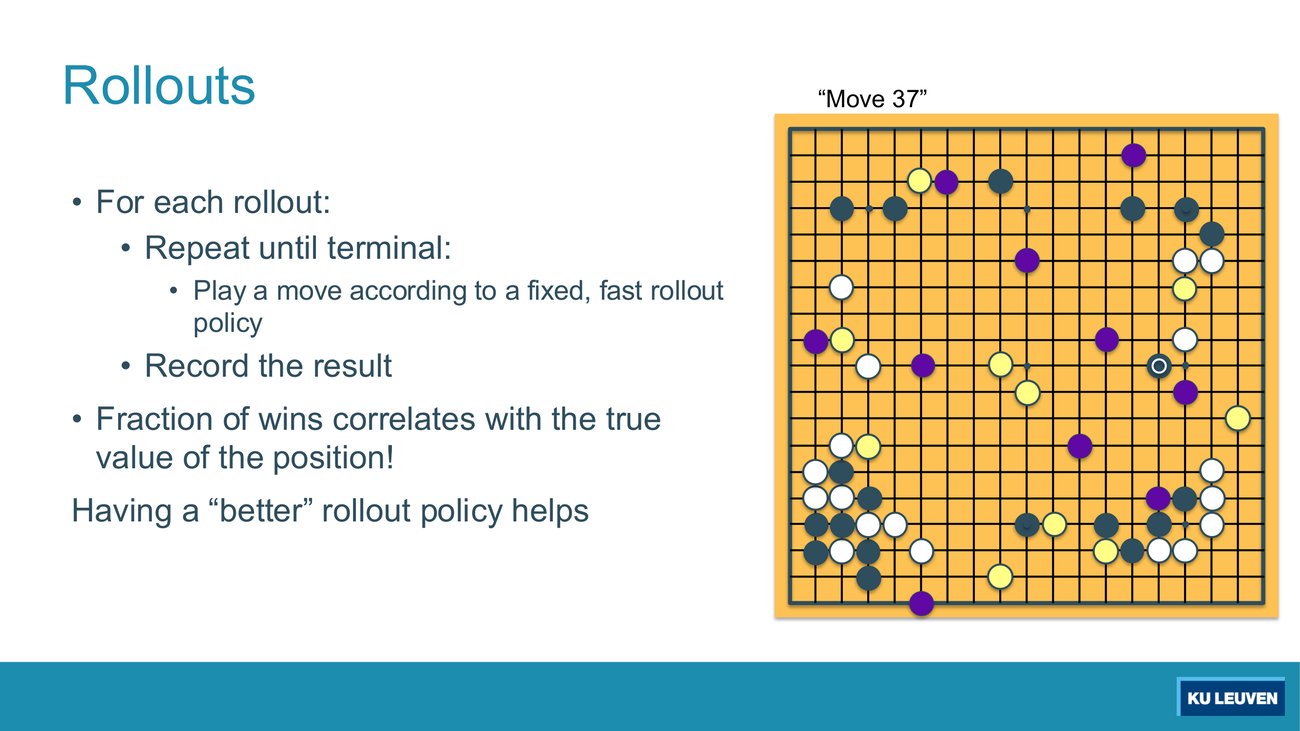
A rollout plays moves from a "simple, fast" policy, which for plain MCTS is close to random. Random play is a terrible model of how the game will actually continue. Why is counting wins under such a policy nevertheless informative, and what is the exact quantity being estimated? Then state the trade-off from p.42 as an inequality in your own terms.
Why it works: a rollout is a sample. If a position is genuinely strong for you, then even unskilled continuations tend to end in your favour more often than not; if it is losing, random play loses more often. The estimate U/N is the sample mean of that win indicator, so it converges to the position's win probability under the rollout policy, and that quantity correlates with the true value of the position. It is not the minimax value, and the deck does not claim it is.
The trade-off: in a fixed time budget T, you get N ≈ T / (cost per rollout) samples. The error on a win-rate estimate shrinks like 1/sqrt(N). A policy that improves the correlation but multiplies the cost by k must therefore buy more than a factor sqrt(k) of accuracy to be worth it, otherwise the extra noise from having fewer samples eats the gain. That is the "tradeoff UCT expansion versus rollout time" line on p.42.
Also worth naming: AlphaGo's improvement was not a cleverer tree rule but a learned policy for choosing which nodes to expand and how to roll out, which is the same lesson as section 6, that the estimate, not the search, is usually the bottleneck.
Exercise session 5, section 3, verbatim (FAI_EXERCISES_Game_Trees.pdf). Archetype A14
Exercise session 5, section 3, gives an expectiminimax tree with A as a MAX node, chance nodes B, C and D, and leaf nodes described as MIN nodes. The two questions are printed as:
What is the value of the nodes B and D (show your calculations)?
Given that you know that MAX node A unambiguously chooses D, what can you say about the values of X and Y?
The stem, verbatim: Consider the following expectiminimax tree (A is a MAX node, the leaf nodes are MIN nodes)
The shape of the answer: one weighted sum per chance node, then the missing probability from the sum-to-one law, then an inequality with a single unknown, solved. "Show your calculations" is in the question text, so the weighted sums must appear on your sheet, not just the results.
B = 0.3(5) + 0.7(1) = 1.5 + 0.7 = 2.2
D = 0.1(5) + 0.9(6) = 0.5 + 5.4 = 5.9
X = 1 − (0.4 + 0.3) = 0.3, by the law that a chance node's arc probabilities sum to one.
C = 0.4(5) + 0.3(9) + 0.3Y = 4.7 + 0.3Y. A chooses D unambiguously, so C < D: 4.7 + 0.3Y < 5.9, giving 0.3Y < 1.2, so Y < 4. B = 2.2 is already far below D and places no constraint.
What earns the marks: the two weighted sums written out in full, because the question says "show your calculations"; X derived from the sum-to-one law rather than treated as a free unknown; and the strict inequality Y < 4, because "unambiguously" rules out the tie at Y = 4, where C = 5.9 = D. All values verified in Python.
B has children 5 and 1 with probabilities 0.3 and 0.7. D has children 5 and 6 with probabilities 0.1 and 0.9. C has three children, 5 with probability 0.4, 9 with probability 0.3, and Y with probability X. A is a MAX node choosing among B, C and D, and it chooses D unambiguously. Find B, D, X and the constraint on Y.
B = 0.3(5) + 0.7(1) = 1.5 + 0.7 = 2.2.
D = 0.1(5) + 0.9(6) = 0.5 + 5.4 = 5.9.
X = 1 − (0.4 + 0.3) = 0.3, forced by the law that the distribution over a chance node's children sums to one.
C = 0.4(5) + 0.3(9) + 0.3Y = 2.0 + 2.7 + 0.3Y = 4.7 + 0.3Y. A chooses D unambiguously, so C < D: 4.7 + 0.3Y < 5.9, hence 0.3Y < 1.2, hence Y < 4. All verified.
Three ways to lose marks here. (1) Taking min or max at B, C or D. (2) Treating X as free: it is determined. (3) Writing Y ≤ 4 instead of Y < 4. The word "unambiguously" is what makes the inequality strict; at Y = 4 exactly, C = 5.9 = D and the choice is a tie, so it is no longer unambiguous. Also note that B never enters the inequality: it is already far below D, so only C constrains anything.
I end up with less than four not less than three but presumably just a small calculation error.(Exercise session, T8), said live while solving this exact question. Y < 4 is what the published solution slides derive, and it is what the arithmetic above gives. Take the lesson rather than the number: the person at the board doubted a correct result because he expected a different one. If you can rebuild 4.7 + 0.3Y < 5.9 from the tree in twenty seconds, you never need to trust a remembered answer.
Exercise session 5, section 4, is the question the session flags as historically confusing. Alice plays a two-player game with Bob. Alice is a maximizer. Bob is also a maximizer, but Alice believes Bob is a minimizer with probability 0.5 and a maximizer with probability 0.5, and Bob is aware of Alice's assumption. Square nodes are outcomes, triangular nodes are Alice's moves, round nodes are Bob's moves. Each node for Alice or Bob contains a tuple: the left value is Alice's expectation of the outcome, the right value is Bob's. Tie-breaking: choose the left branch.
The mechanism, stated once so you never have to re-derive it under time pressure:
Exercise session 5, section 4, verbatim (FAI_EXERCISES_Game_Trees.pdf). Archetype A15
Alice is playing a two-player game with Bob in which they move alternately. Alice is a maximizer. Although Bob is also a maximizer, Alice believes Bob is a minimizer with probability 0.5, and a maximizer with probability 0.5. Bob is aware of Alice's assumption. In the game tree below, square nodes are the outcomes, triangular nodes are Alice's moves, and round nodes are Bob's moves. Each node for Alice/Bob contains a tuple, the left value being Alice's expectation of the outcome, and the right value being Bob's expectation of the outcome. Tie-breaking: choose the left branch.
The tree, as printed: Alice's node B chooses between an outcome of 4 and a Bob node whose children are 1 and 9. Bob's node E has children 1, 13 and 10. Bob's node D has children 8 and X.
What are the values for the tuples (Ba, Bb) and (Ea, Eb) in the above game tree?
Choose the appropriate value for Daand
Choose the appropriate value for Db, from the printed options A. 8, B. X, C. 8 + X, D. 4 + 0.5X, E. min(8, X), F. max(8, X).
Bob's node under B has children 1 and 9. Bob really maximises, so its right component is max(1, 9) = 9. Alice's belief is a 50/50 mixture over two behaviours, so her component is (1 + 9)/2 = 5. The node is (5, 9).
At Alice's node B she compares her own readings, 4 for the outcome leaf and 5 for the Bob node, takes 5, and copies the winning child's whole tuple upward: (Ba, Bb) = (5, 9). Alice thinks the line is worth 5; it is actually worth 9.
E has children 1, 13 and 10. Eb = max = 13. Ea = (Bob minimising, 1, plus Bob maximising, 13) / 2 = 7, so (Ea, Eb) = (7, 13). The child 10 contributes nothing, because the mixture is over two behaviours and not over the three children.
What earns the marks: never mixing two children's tuples (a tuple describes one real board state), averaging only Bob's minimising and maximising choices, and stating the tie-break rule when you use it.
Choose the appropriate value for Da, where Bob's node D has children 8 and X:
Choose the appropriate value for Db, same options:
Alice's node B chooses between the outcome 4 and a Bob node whose children are 1 and 9. Bob's node E has children 1, 13 and 10. Bob's node D has children 8 and X. Compute (Ba, Bb) and (Ea, Eb), then choose Da and Db from the printed options: A. 8, B. X, C. 8 + X, D. 4 + 0.5X, E. min(8, X), F. max(8, X).
The Bob node under B has children 1 and 9. Bob's own value is max(1, 9) = 9. Alice's value is the average of Bob minimising (1) and Bob maximising (9), that is (1 + 9)/2 = 5. So that node is (5, 9).
(Ba, Bb): Alice compares her own readings, 4 for the leaf and 5 for the Bob node, and picks 5. The whole tuple travels upward, so (Ba, Bb) = (5, 9). Alice thinks the line is worth 5; it is in fact worth 9.
(Ea, Eb): Bob maximises over 1, 13, 10, so Eb = 13. Alice averages Bob's minimising choice (1) with his maximising choice (13): (1 + 13)/2 = 7. So (Ea, Eb) = (7, 13).
Da = 0.5(8) + 0.5(X) = 4 + 0.5X, option D. Db = max(8, X), option F.
The trap in E. One of the three children contributes nothing: the one that is neither Bob's maximising choice nor his minimising choice, here the rightmost child, 10. Alice's belief is a mixture over two behaviours, minimise and maximise, not a uniform distribution over children, so a middling child is never selected under either behaviour. Averaging all three children gives (1 + 13 + 10)/3 = 8, which is wrong. Read the children by role, not by position: E is drawn with 1, 13 and 10 from left to right, so the max is the middle one and the ignored child is the last one.
the average of one and 13 is seven, right? Not six.(Exercise session, T8), on node E. Two lessons in one line. First, the mixture is over 1 and 13 only, not over all three children. Second, the arithmetic slip that gets corrected out loud is (1 + 13)/2 read as 6, the sort of error that costs a mark on an otherwise perfect tree. Under exam pressure, write the sum before you halve it.
in the past these kind of things sometimes were exam questions and if it was like the first time that you saw this kind of description, people were just confused.(Exercise session, T8), on why this question is in the session at all. Treat it as a stated exam signal: non-standard tree descriptions have been examined. The defence is a fixed reading procedure, which the session states as: work out what a game state is and how many numbers describe it, then work out for each internal node who is acting, then work out what each actor maximises or minimises or averages. Three-player minimax (exercise session 5, section 2) is the same drill with a different twist: leaves carry a tuple with one utility per player, every layer belongs to one player and maximises that player's own component, turns go clockwise, and the winning child's whole tuple is copied upward. There is no minimisation anywhere in that tree, and therefore no alpha-beta pruning either.
Exercise session 5, section 5, verbatim (FAI_EXERCISES_Game_Trees.pdf). Archetype A16
Exercise session 5, section 5, prints a partial Monte Carlo tree whose nodes are annotated with UCB values, and states that Nodes that have not been full expanded yet have an edge exiting them without a destination node.
The two tasks are:
Indicate which node the next random rollout would occur at.
Assuming the next random rollout results in a loss, indicate for each shown UCB value whether this value would increase, decrease or stay the same.
The classic mistakes. (1) Descending to a terminal leaf instead of stopping at the first node that still has an unexpanded edge, which can be a node that already has children. (2) Marking only the nodes on the path and forgetting that every sibling of a path node rises, including the children the expanded node already had. (3) Assigning a UCB value to the root. (4) Assuming a loss lowers everything: four of the six changed values go up.
Question 1, with options supplied so you can self-test. In the published tree the root has 13 rollouts and children 3/5, 2/4 and 1/4 printed 1.61, 1.63 and 1.38; the 2/4 child has children 1/2 and 0/1 printed 1.68 and 1.67; the 1/2 node has one child printed 1.18 and still shows an edge leaving it with no destination. At which node does the next random rollout occur?
Counts after the loss: the new node c is 0/1, the selected 1/2 node becomes 1/3, the middle child becomes 2/5, the root becomes 6/14.
Decrease (2), the nodes on the selected path: the 1/2 node, 1.68 to 1.37, and the middle child, 1.63 to 1.43.
Increase (4), the siblings of nodes on the path: the existing 0/1 child of the selected node, 1.18 to 1.48, because c is on the path and this node is c's sibling; the 0/1 sibling of the selected node under the middle child, 1.67 to 1.79; and the root's other two children, 3/5 from 1.61 to 1.63 and 1/4 from 1.38 to 1.40.
Unchanged: everything under the root's first and third children, that is 2.27, 1.77, the two 2.18 labels, and the 1.18 and 1.67 pair with the 1.18 below them. Two labels read 1.18 and two read 1.67, so identify nodes by position, not by value. The root has no UCB1 at all, since it has no parent, although its counter goes from 13 to 14.
What earns the marks: four increases and two decreases, the reason stated once (a node's exploration term rises whenever its parent is visited and it is not), and the root left blank rather than given a value. All values verified in Python with C = sqrt(2) and natural logarithms. Step it yourself in viz-uncertainty.html.
In the session's tree the root has 13 rollouts and three children recorded 3/5, 2/4 and 1/4, with printed UCB values 1.61, 1.63 and 1.38. The middle child (2/4) has two children of its own, 1/2 and 0/1, printed 1.68 and 1.67. The 1/2 node already has one child, 0/1, printed 1.18, and still has unexpanded moves, drawn as edges with no destination node. The right child (1/4) has children 0/2 and 0/1, printed 1.18 and 1.67, and the 0/2 node has a child printed 1.18. (a) Trace the selection. (b) Assume the rollout is a loss and classify every printed UCB value in the tree as increased, decreased or unchanged. (c) Verify one of the printed numbers from the formula.
(a) At the root, pick the largest UCB1: 1.63, the middle child. At the middle child, pick the larger of 1.68 and 1.67: the 1/2 node. That node still has an edge exiting to nothing, so it is not fully expanded even though it already has one child. Stop there, add a new child c, and roll out from c.
(b) After a loss the counts become 0/1 at the new node c, 1/3 at the selected node, 2/5 at the middle child and 6/14 at the root. Those updated visit counts, 3, 5 and 14, are exactly the numbers the solution slide writes over the struck-out ones.
| Node | Printed | After | Direction and reason |
|---|---|---|---|
| Selected node, 1/2 to 1/3 (its parent 4 to 5) | 1.68 | 1.37 | decrease, on the path |
| Middle child, 2/4 to 2/5 (its parent 13 to 14) | 1.63 | 1.43 | decrease, on the path |
| Existing child 0/1 of the selected node (parent 2 to 3) | 1.18 | 1.48 | increase, sibling of the new node c |
| Sibling 0/1 of the selected node, under 2/4 (parent 4 to 5) | 1.67 | 1.79 | increase, sibling of a path node |
| Root's first child 3/5 (parent 13 to 14) | 1.61 | 1.63 | increase, sibling of a path node |
| Root's third child 1/4 (parent 13 to 14) | 1.38 | 1.40 | increase, sibling of a path node |
Four increases and two decreases, which is what the solution slide marks. Unchanged: 2.27 and 1.77 under the root's first child, the two 2.18 labels one level below them, and, under the root's third child, its 1.18 and 1.67 together with the 1.18 one level further down. Note that two different labels read 1.18 and two read 1.67; only the copies whose parent lies on the selected path move, so identify these nodes by position rather than by value. The root itself has no UCB1, since it has no parent, although its counter goes from 13 to 14.
The rule that catches the third row is worth stating once: a node's exploration term rises whenever its parent is visited and it is not. The newly added node c is on the path, so c's siblings, that is the already-existing children of the node you just expanded, rise as well. "Siblings rise" is the whole rule only if you remember that c counts as a node on the path. All values verified with C = sqrt(2) and natural logarithms.
(c) Middle child: 2/4 + sqrt(2)·sqrt(ln 13 / 4) = 0.5 + 1.41421·sqrt(2.56495/4) = 0.5 + 1.41421(0.80077) = 0.5 + 1.13245 = 1.6325, printed as 1.63. The same constant reproduces the other twelve labels in that figure, which carry nine distinct values: 1.61, 1.63, 1.38, 2.27, 1.77, 1.68, 1.67, 1.18 and 2.18.
it's important that you can put together these algorithms and that you can reason about them. For example, if you are given a number of ingredients that you can say something about the properties along these four uh dimensions or for example give a counterargument if something is not optimal... It's also important that you can execute and simulate these algorithms in a pen and paper uh version on a small scale.(Lecturer, T4), about search algorithms generally, and the standard this Part is graded against. "Execute and simulate on a small scale" is literally what all three archetypes above ask: one expectimax tree, one mixed-belief tree, one UCT iteration, all small enough to do by hand and all requiring the mechanism rather than a memorised result.
Time budget: about nine minutes per point across a three-hour paper split into a theory half handed in before the exercise half is issued. A full UCT iteration with a rise/fall table is well inside that if the formula is automatic.
the theory exam... tests both for factual knowledge as well as for synthetic knowledge... we also want to see that you can uh bring things across different chapters uh together because as you know by now uh the course is largely incremental.(Lecturer, T9). For this Part the cross-chapter joins that are most likely to be asked are: chance node versus min node (Part 7), why alpha-beta does not transfer (Part 7), evaluation functions and the depth limit (Part 7), stochastic environments (Part 2), and the chance node becoming the q-state of an MDP (Part 9).
| Term | Precise definition | Plain paraphrase | Exam phrasing |
|---|---|---|---|
| Chance node | A node whose value is the probability-weighted sum of its children's values, used for any outcome out of the agent's control (pp.5, 16). | A layer where nobody chooses; the world rolls. | "Chance nodes are like min nodes but the outcome is uncertain" (p.5) |
| Expectimax | Search over a tree of MAX and chance layers; MAX takes maxima, chance nodes take expectations (pp.5, 8). | Minimax with the opponent replaced by an average. | "compute the average score under optimal play" (p.5) |
| exp-value | Initialise v = 0; for each successor, v += probability(successor) × value(successor); return v (pp.8, 9). | Add up each child's value times its chance. | "What is the value of the nodes B and D (show your calculations)?" (exercise session 5 §3) |
| Expected value | The average of a function of a random variable, weighted by the probability distribution over outcomes (p.15). | Sum of value times probability. | "v = (1/2) (8) + (1/3) (24) + (1/6) (-12) = 10" (p.9) |
| Dangerous optimism | Assuming chance when the world is adversarial (p.19); measured as Won 1/5, Avg. Score −303 (p.21). | Averaging over a monster that always picks the worst branch. | the Expectimax Pacman row, Adversarial Ghost column (pp.20-21) |
| Dangerous pessimism | Assuming the worst case when it is not likely (p.19); measured as Won 5/5, Avg. Score 493 (p.21). | Running from a rabbit; you survive, you waste time. | the Minimax Pacman row, Random Ghost column (pp.20-21) |
| Expectiminimax | Search over mixed layers where the environment is an extra random-agent player that moves after each min or max agent, and each node computes the appropriate combination of its children (p.27). | Max, then dice, then min, then dice. | "Consider the following expectiminimax tree (A is a MAX node, the leaf nodes are MIN nodes)" (exercise session 5 §3) |
| Rollout | A game played to termination from a state using a fixed, fast rollout policy, with the result recorded as a win or a loss (pp.31, 41). | Finish the game quickly and badly, then note who won. | "Evaluation by rollouts" (pp.31, 42) |
| Selective search | Exploring parts of the tree that will help improve the decision at the root, regardless of depth (pp.31, 42). | Spend effort where it changes the answer. | "explore parts of the tree that will help improve the decision at the root" (p.31) |
| MCTS | Monte Carlo tree search: the combination of evaluation by rollouts and selective search (p.31). | Sample instead of evaluate; grow the tree where it matters. | "MCTS combines two important ideas" (pp.31, 42) |
| N(n), U(n) | N(n) is the number of rollouts from node n; U(n) is the total utility of rollouts (e.g. # wins) for Player(Parent(n)) (p.37). | How often we looked here, and how often it went well. | "U(n) = total utility of rollouts (e.g., # wins) for Player(Parent(n))" (p.37) |
| UCB1 | UCB1(n) = U(n)/N(n) + C × sqrt(log N(Parent(n)) / N(n)); an upper confidence bound combining a win rate with an exploration bonus (p.37). | How good it looks, plus how little we know about it. | "indicate for each shown UCB value whether this value would increase, decrease or stay the same" (exercise session 5 §5) |
| UCT | MCTS version 2.0: repeatedly apply UCB down to a not-fully-expanded node, add a child, roll out, update counts to the root; finally choose the action leading to the child with highest N (p.38). | Select, expand, simulate, back up; then play the most-visited move. | "Choose the action leading to the child with highest N" (p.38) |
| Exploration term | C × sqrt(log N(Parent(n)) / N(n)): falls when n is visited, rises when a sibling is visited, since only the parent's count grows (p.37). | The bonus for being the one we have not tried lately. | "the siblings basically are going to ever so slightly increase" (exercise session, T8) |
Constructed, in the sample paper's format. Built from the UCT row of this term box, p.38
A UCT search runs out of time. Which child of the root does it play?
Choose the action leading to the child with highest N. B is the trap and the commonest wrong answer: a child can carry a high win rate on very few rollouts, which is exactly the situation UCB1 exists to distrust (see the 6/10 versus 61/100 comparison in section 14). A returns the node you most want to explore next, which is a different question, and by design it favours the least visited child. D mixes the two, since U(n) grows both when a child is good and when it is merely visited often. Under UCT the visit count is the accumulated verdict of every previous selection, which is why it, and not the win rate, is the output.
Every numeric answer in this chapter was computed and checked in Python: the p.9 and p.10 expectimax values, the p.11 pruning bound, the p.15 expectation, the p.17 quiz probabilities, the p.29 three-tree comparison, the p.20-21 score inference, and every UCB1 value for the p.39 tree and for the exercise-session tree, using C = sqrt(2) and natural logarithms. The deck prints C as a symbol; the constant is inferred, and stays marked as inferred throughout, from the exercise-session solutions, where it reproduces all thirteen printed UCB labels (nine distinct values).
Chapter index: index.html · Previous: Part 7, Game Trees · Next: Part 9, Markov Decision Processes · Search by question: question-index.html