CSPs as a special search problem, constraint graphs, backtracking, filtering by forward checking and by arc consistency, the AC-3 algorithm, k-consistency, variable and value ordering, exploiting graph structure, value symmetry, and constraint optimisation.
Printing reveals every hidden answer automatically. On screen, use Show all answers in the tier bar at the top.
Printed copy: all task answers below are revealed. On screen they are hidden behind a click, which is how you should use them first.
Deck pp.3 to 6 replay Part 4 and Part 5 in four slides: a node in a search tree is an entire path through the state space graph (p.3), informed search is guided towards the goal while uninformed search spreads out all over the place (p.4), a heuristic estimates how close a state is to a goal (p.5), and A* orders the queue by f(n) = g(n) + h(n) and is optimal for trees or graphs given an admissible or consistent heuristic (p.6). That is the baggage you carry in.
Deck p.10 then draws the distinction that motivates the whole Part. It splits search problems in two, under a fixed set of assumptions printed at the top of the slide: a single agent, deterministic actions, fully observed state, discrete state space.
Read that literally. In a CSP you do not care how you arrived at the assignment. Two search paths that end in the same complete assignment are the same answer. That single observation is worth an enormous amount of pruning, and section 6 shows exactly where it is cashed in.
Deck p.11 gives the definition, contrasting it with the generic search problems of Part 3:
The slide's own summary of what you gain: this is a "simple example of a formal representation language" and it "allows useful general-purpose algorithms with more power than standard search algorithms". The power comes from the fact that the solver can now read the structure of the problem, because the state is factored and the goal test is declarative rather than a black-box function.
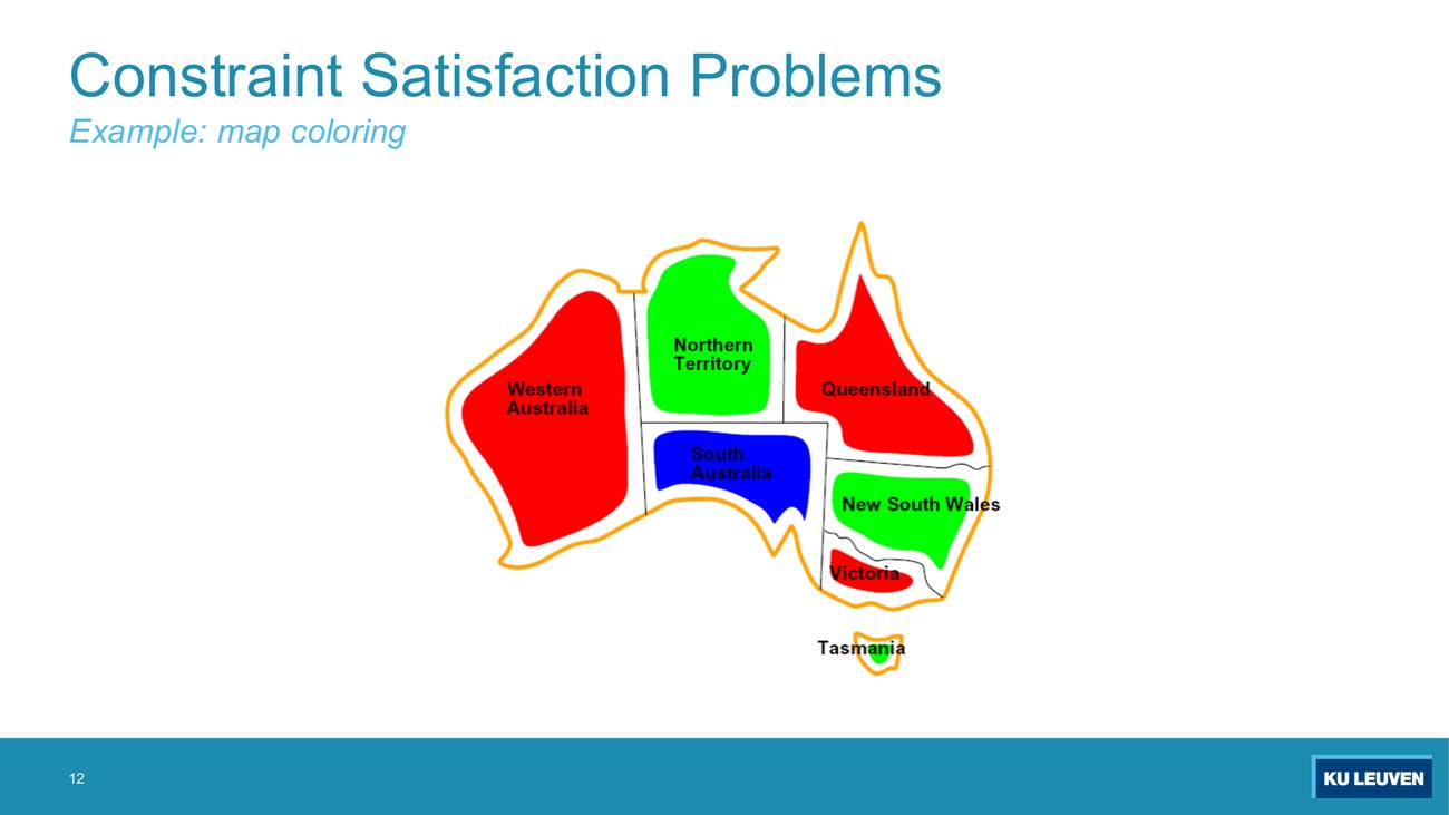
Deck pp.12 and 13 introduce the example that the rest of the deck uses for almost every algorithm: colour the regions of Australia so that adjacent regions differ.
Write down the full list of binary constraints implied by this map, using the region abbreviations WA, NT, SA, Q, NSW, V, T. How many are there, and which region appears in none of them?
Nine constraints: WA≠NT, WA≠SA, NT≠SA, NT≠Q, SA≠Q, SA≠NSW, SA≠V, Q≠NSW, NSW≠V. Tasmania (T) appears in none of them, because it is an island and shares no border. Verified by enumerating the adjacency list used for every trace in this chapter.
Why it matters: SA occurs in five of the nine, T in zero. Those two extremes drive section 11 (the degree heuristic picks SA first) and section 12 (T is a separate connected component and can be solved on its own).
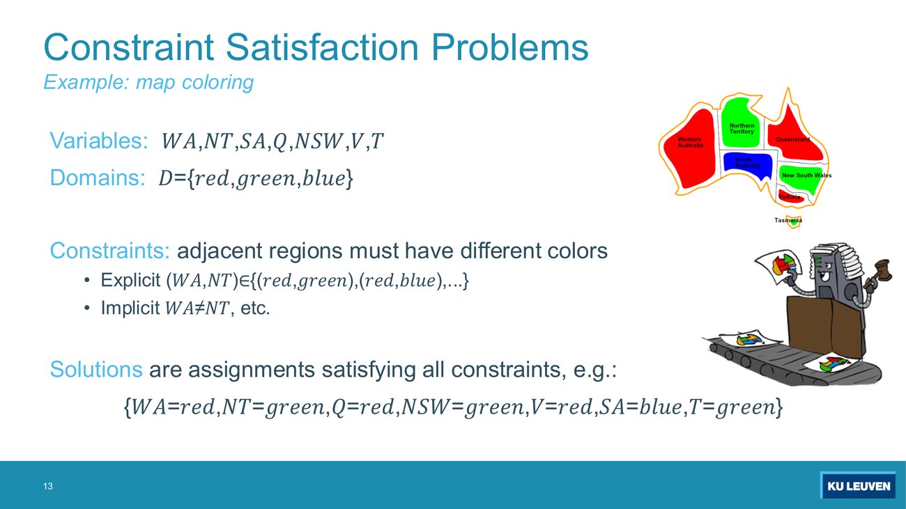
The slide gives the explicit form of one constraint as (WA,NT) ∈ {(red,green),(red,blue),...} and the implicit form as WA ≠ NT. Write out the explicit set in full. Then say how many solutions the whole seven-region CSP has.
Explicit set, six ordered pairs: {(red,green), (red,blue), (green,red), (green,blue), (blue,red), (blue,green)}. It is the complement of the three equal pairs inside the nine possible ordered pairs. "Explicit" means enumerating the allowed tuples; "implicit" means writing a formula that generates them. They denote the same relation, and the choice affects only how much you have to write.
18 solutions. Computed by enumerating all 37 = 2187 assignments and testing the nine constraints: 18 satisfy all of them. Six of those are the mainland colourings, and Tasmania multiplies each by 3 because it is unconstrained. Section 12 uses that number again.
Exercise session 4, opening illustration, verbatim from FAI_Exercise_CSP.pdf p.1
"There are three countries aligned on a fictive map (A,B and C; B neighbours A and C). Colour the countries red or green, while ensuring that the following requirements are met: 1. Neighbouring countries should have different colours. 2. Country A should not be coloured red."
The sheet then works the formalisation in four named steps, in this order: decision variables, initial domains, constraints, constraint graph. Produce all four before reading on. Every later answer in session 4 opens with the same four steps, so this is the shape the marker is looking for.
Decision variables: "We define a decision variable for every country, so we have 3 variables: A, B and C".
Initial domains: "Each country has to be coloured red or green, so the initial domain of every decision variable is the set of values 'red' and 'green': [A={red,green}, B={red,green}, C={red,green}]".
Constraints: (1) A ≠ B and B ≠ C; (2) A ≠ red. Note which is which: the first requirement becomes two binary constraints, one per adjacent pair, and the second is a single unary constraint.
Constraint graph: three nodes A, B, C; an edge A to B labelled A ≠ B and an edge B to C labelled B ≠ C; the unary A ≠ red written at the node A, not as an edge. The sheet's own words: "every variable is a node in the graph, and there is an edge between every two variables that share a constraint (with the edge labelled by the constraint)". There is no edge A to C, because A and C share no constraint even though both border B.
What earns the marks: writing the domains as one bracketed vector rather than three separate lines (that vector is what you then carry down every node of the search tree in section 7), labelling each edge with its constraint, and putting the unary constraint at its node. Verified: the CSP has exactly one solution, A = green, B = red, C = green, which is the sheet's own closing sentence, "There is thus only one correct assignment: A=green, B=red and C=green."
Deck pp.14 and 15 model the same puzzle twice. This is the deck's demonstration of the Part 3 slogan that formulation decides difficulty.
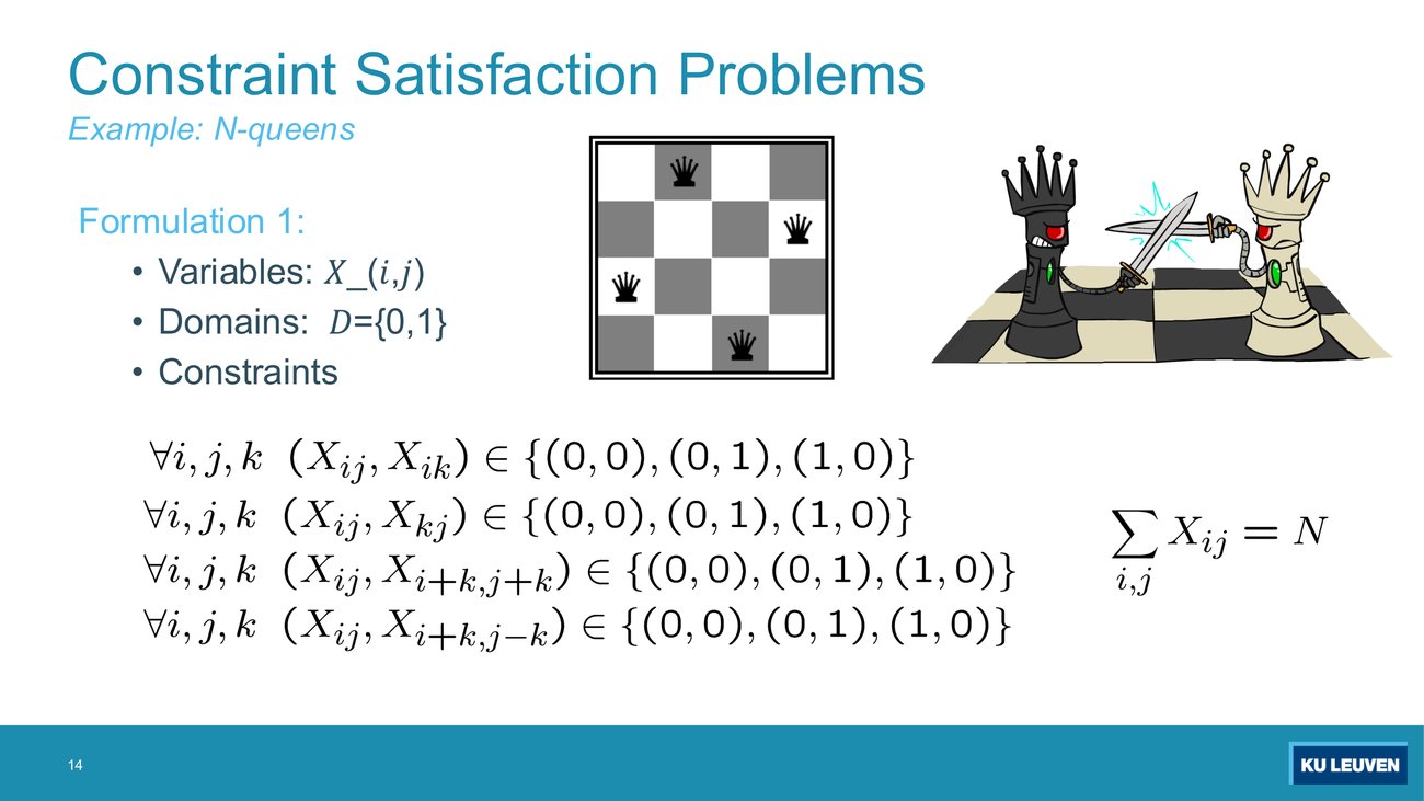
Formulation 1 uses one boolean variable per square, Xi,j ∈ {0,1}, four families of pairwise constraints, and the global constraint ∑i,j Xi,j = N. For N = 8, how many complete assignments does the search space contain, and what is the specific defect of this encoding?
264 = 18,446,744,073,709,551,616 complete assignments (64 boolean variables). The defect is that the encoding does not build in what you already know: exactly one queen per column and per row. Instead it must be stated, and stated as a global sum constraint over all 64 variables, which is not binary and therefore does not fit the binary constraint graph machinery of section 4 without a hypergraph (a graph in which one constraint node may join more than two variables at once).
Compare with formulation 2 on the next slide: 88 = 16,777,216 assignments, a factor of about 1.1 × 10¹² smaller. Same puzzle, same answers, different amount of work. That is the Part 3 point restated in numbers.
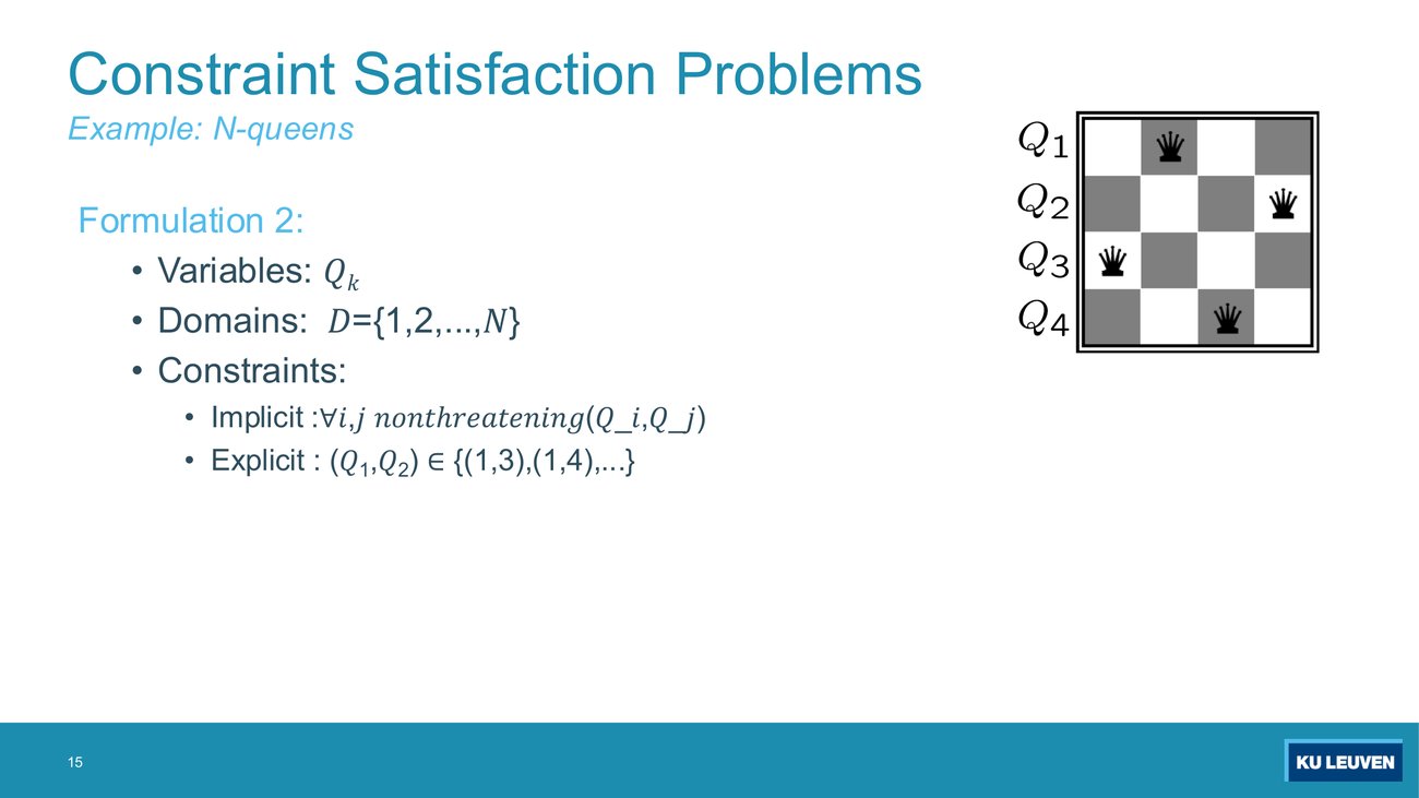
Formulation 2 has one variable Qk per column with domain {1,...,N}. Which of the four original constraint families has now disappeared completely, and why? Write the remaining constraints as formulas in Qi and Qj.
The column constraint disappears, and so does the sum constraint: because there is exactly one variable per column and every variable must take exactly one value, "exactly one queen per column" is enforced by the representation itself and can no longer be violated. That is what a good formulation does: it makes an entire class of illegal states unrepresentable rather than merely forbidden.
What remains, for all i ≠ j: Qi ≠ Qj (no shared row) and |Qi − Qj| ≠ |i − j| (no shared diagonal). The slide writes this as the implicit predicate nonthreatening(Qi,Qj) and gives the explicit alternative (Q1,Q2) ∈ {(1,3),(1,4),...}.
Deck p.16 defines the object every later algorithm reads: a binary CSP is one where each constraint relates at most two variables, and its binary constraint graph has variables as nodes and constraints as arcs. The slide states the payoff directly: "General-purpose CSP algorithms use the graph structure to speed up search. E.g., Tasmania is an independent subproblem!" And it flags the escape hatch: "For higher order constraints, hyper-graph representations might be used".
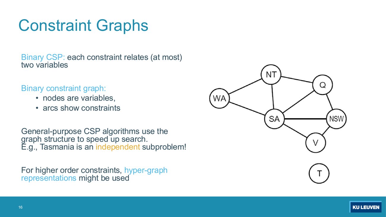
A student says: "the constraint graph tells me which regions are adjacent, so it is just the map redrawn". Give one thing the graph records that the map does not, and one thing the map records that the graph deliberately throws away.
The graph records which variables share a constraint, whatever the constraint is. For this problem the constraints happen to be "different colour", but the same graph shape would appear for "must be within 2 of each other" or any other binary relation. The graph is an abstraction over constraint scopes, not over geography, and every algorithm in sections 8 to 12 uses only the scopes.
The graph throws away geometry: areas, shapes, distances, and which side of a border a region lies on. That is the point. It also throws away the content of each constraint, which is why arc consistency has to consult the actual relation again when it revises a domain.
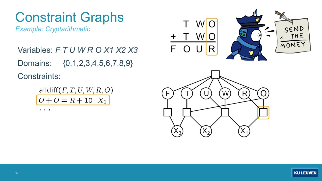
The slide prints alldiff(F,T,U,W,R,O) and the first column constraint O + O = R + 10·X1, then "...". Write the other three column constraints, using the carries X1, X2, X3. Then say why the picture has square nodes at all.
W + W + X1 = U + 10·X2, then T + T + X2 = O + 10·X3, then X3 = F. Read the addition column by column from the right, exactly as in school arithmetic; each carry becomes its own variable with domain {0,1} in effect.
The squares are the constraints themselves. Count the scopes: the highlighted first column O + O = R + 10·X1 links three variables (O, R, X1), the two middle columns link four each (W, X1, U, X2 and T, X2, O, X3), and the last is X3 = F over two. Any constraint whose scope is larger than two cannot be drawn as an edge between two nodes, which is the whole reason this picture is a hypergraph: you draw the constraint as a node (the square) and connect it to every variable in its scope. The alldiff square at the top touches all six letters. The introduction of the carry variables is what keeps the arithmetic constraints down to four variables each instead of one giant relation.
Deck p.18 does the same for Sudoku, with no figure in this pack: variables are the open squares, domains are {1,...,9}, and the constraints are "9-way alldiff for each row", the same for each column and each region, with the slide adding the alternative "(or can have a bunch of pairwise inequality constraints)". That parenthesis is the general escape route: any alldiff over k variables can be rewritten as C(k,2) binary disequalities, at the cost of weaker propagation.
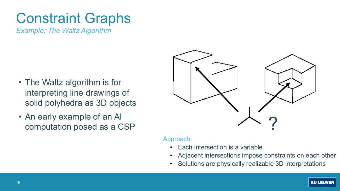
The slide gives the approach in three bullets: "each intersection is a variable", "adjacent intersections impose constraints on each other", "solutions are physically realizable 3D interpretations". What are the values, and what exactly is the constraint between two adjacent intersections?
The values are the physically possible labellings of the lines meeting at that junction: each line at a junction receives a label, only certain combinations of labels can occur at a corner of a real solid, and so the domain of a junction variable is its catalogue of legal local interpretations. The named label set (convex, concave, occluding) and the catalogue of legal trihedral corners are textbook Huffman-Clowes line labelling (background beyond the deck, not examinable).
The constraint is agreement on the shared line. Two adjacent junctions are joined by one line segment, and that segment gets a label from each end. The constraint says the two labels must be the same. This is a binary CSP, and the slide's own point is that a 1970s vision program was already a CSP: the same "?" ambiguity shown at the bottom of the slide is resolved by propagation, not by search over 3D models.
Deck p.21 classifies by variable type:
Deck p.22 classifies by constraint arity: unary constraints involve a single variable and are "equivalent to reducing domains", with SA ≠ green as the example; binary constraints involve pairs, with SA ≠ WA; higher-order constraints involve three or more, "e.g., cryptarithmetic column constraints". The slide then introduces preferences, also called soft constraints: "for example, red is better than green", "often representable by a cost for each variable assignment", which "gives constrained optimization problems". Section 14 picks that thread back up.
The unary line deserves emphasis, because it is the first move in every exercise: a unary constraint is not something you check during search, it is something you apply once to shrink the domain before search starts. Exercise session 4 requires exactly this as the first step of the tree-structured problem ("indicate the domain of each variable after applying unary constraints").
Deck p.23 lists real-world CSPs: assignment problems (who teaches what class), timetabling (which class is offered when and where), hardware configuration, spreadsheets, transportation scheduling, factory scheduling, circuit layout, fault diagnosis, "and a lot more". The closing line points at the boundary of the technique: the slide prints "Many real-world problems involve real-valued variables" with an arrow to "Mathematical programming".
Deck p.25 casts a CSP as an ordinary search problem so that Part 4's algorithms apply unchanged:
The slide is honest about what follows: "We'll start with the straightforward, naïve approach, then improve it".
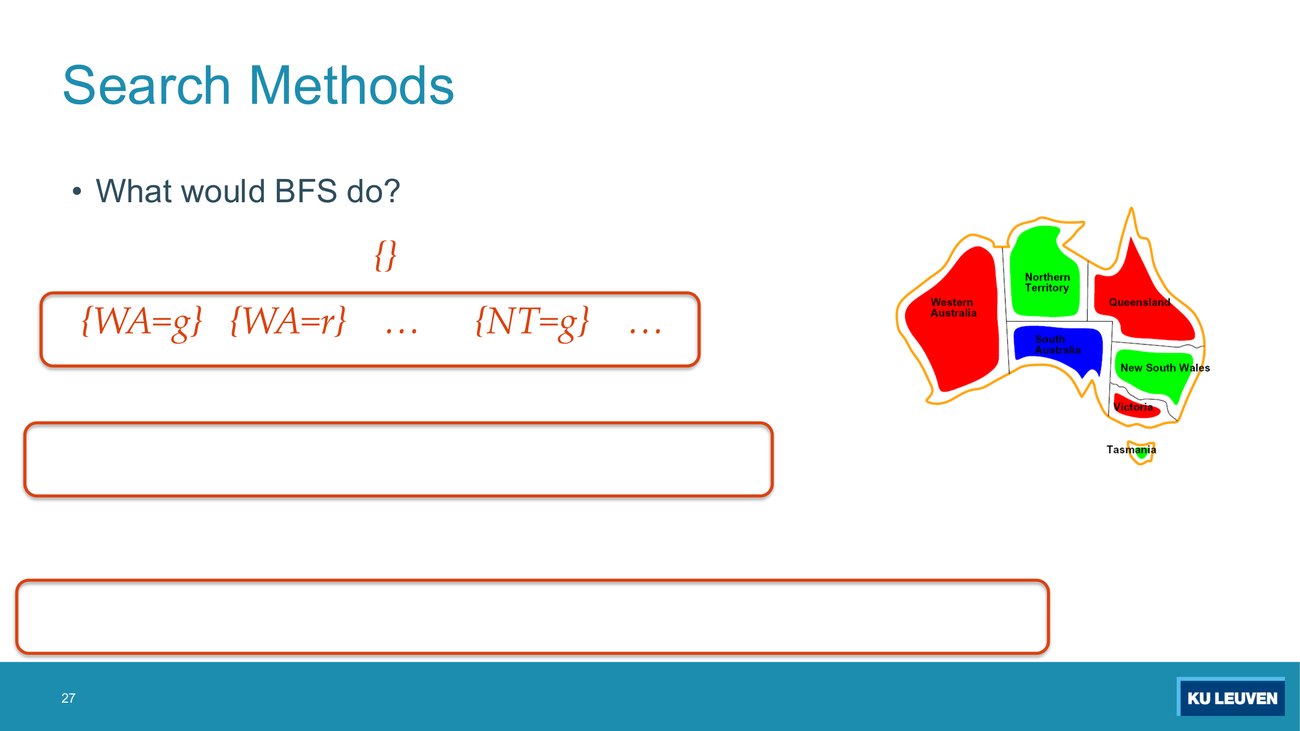
Animation build: the two lower rounded boxes are empty in this PDF export. They are outlined in the same style as the filled level-1 box above them, so they are the next two frontier levels of the same breadth-first walk; that reading is an inference from the slide layout, not from printed text. Treat the figure as a predict-what-appears exercise.
The root is {} and the first box shows {WA=g} {WA=r} ... {NT=g} .... Predict the size of each of the two empty boxes for the seven-variable, three-colour Australia CSP, and then count the leaves of the whole tree. Compare that count with the number of distinct complete assignments.
Level 1 holds n·d = 7 × 3 = 21 nodes, which is what the visible box shows: breadth-first search (BFS) is free to assign any variable first, so both {WA=g} and {NT=g} appear side by side. Level 2 holds n(n−1)d2 = 7 × 6 × 9 = 378 nodes, and level 3 holds 7·6·5·27 = 5670.
Leaves: n! · dn = 5040 × 2187 = 11,022,480, but there are only dn = 37 = 2187 distinct complete assignments. Every assignment is reached 5040 times, once per ordering of the variables. The n! factor is pure waste, and it is exactly what idea 1 on p.31 removes. All numbers computed directly.
Deck p.28 adds "What would DFS do?" beside the BFS question, and p.29 sends you to an interactive demo of map colouring with DFS at the Carnegie Mellon URL printed on the slide. The answer the deck is steering you to: DFS is far better than BFS here because every solution sits at the same depth n, so BFS's advantage (finding shallow goals first) is worth nothing, while its memory cost is catastrophic.
Deck p.31 states the two ideas that turn DFS into backtracking search. Both are consequences of the identification insight from p.10.
The slide's definition, which is also the exam-ready one-liner: "Depth-first search with these two improvement is called backtracking search (not the best name)". And the scale claim: "e.g., can solve n-queens for n ≈ 25".
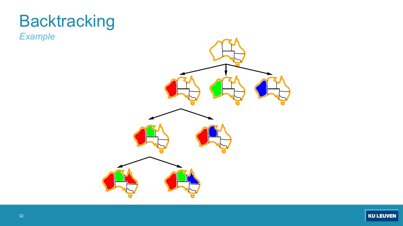
Animation build: this frame shows the tree only along its leftmost branch. Later builds continue the walk. Read it as the state of the search after three expansions: the root, then WA = red, then {WA = red, NT = green}.
The root has three children (WA = red, green, blue). The node WA = red has only two children, and the node {WA = red, NT = green} also has only two. Name the branches that are missing at each of those two nodes, say which of the two ideas from p.31 removed them, and then predict which node the search visits next.
Missing at WA = red: the branch NT = red, because it violates WA ≠ NT. Missing at {WA=red, NT=green}: the branch Q = green, because it violates NT ≠ Q. Both are removed by idea 2, checking constraints as you go: the value is never added to the assignment, so no node is created for it. Idea 1 is what makes each level assign one fixed variable instead of any of the seven.
Next node: depth-first, leftmost-first, so the search descends from {WA=red, NT=green, Q=red} and assigns the next variable (NSW), trying red first and rejecting it because Q ≠ NSW, then green. Running plain backtracking with variable order WA, NT, Q, NSW, V, SA, T and value order red, green, blue reaches a solution with no backtracking at all: {WA=r, NT=g, Q=r, NSW=g, V=r, SA=b, T=r}, after only four rejected value tries. Verified by executing the algorithm.
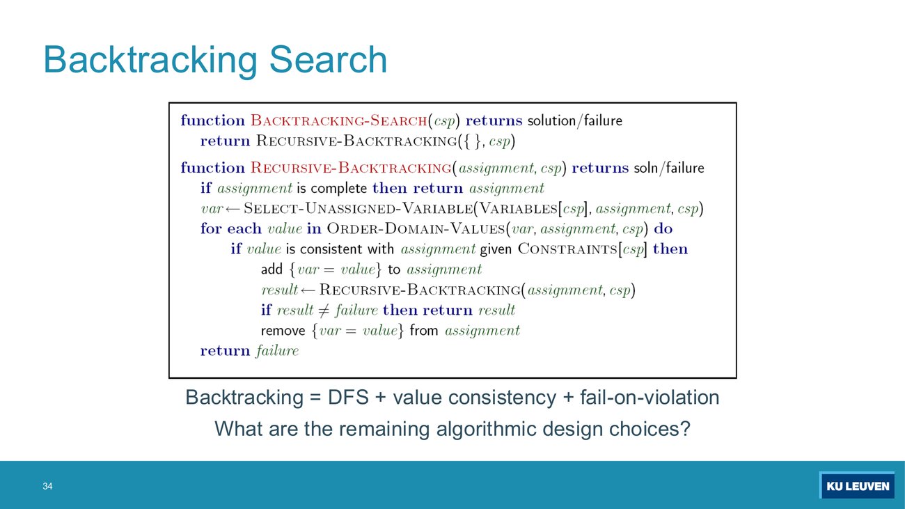
The slide asks "What are the remaining algorithmic design choices?". Point at the two lines of the pseudocode that are the answer, and name the section of this chapter that fills each one in.
Line var ← SELECT-UNASSIGNED-VARIABLE(...) is the variable-ordering hook, filled in by section 11 with minimum remaining values (MRV) and the degree heuristic. Line for each value in ORDER-DOMAIN-VALUES(...) is the value-ordering hook, filled in by section 11 with the least constraining value (LCV).
The third choice is not a named subroutine here: it hides inside if value is consistent with assignment. Strengthening that test from "does not conflict with what is already assigned" to "does not empty a neighbour's domain" is filtering, sections 8 and 9. Deck p.35 lists all three: filtering ("can we detect inevitable failure early?"), ordering ("which variable should be assigned next? in what order should its values be tried?"), and structure ("can we exploit the problem structure?"), under the banner "General idea: try to detect failure early on".
Exercise session 4, exercise 1, task 1, verbatim from FAI_Exercise_CSP.pdf p.2 (archetype A7)
"Consider the following variant of the 4 houses problem: There are 4 families A, B, C and D living in 4 different houses, numbered 1, 2, 3 and 4. C lives in a house with a higher number than the house in which D lives. D lives next to A, in a house with a lower number. There is at least one house between the houses of D and B. C does not live in the house with number 3. B does not live in the house with number 1. Now solve the following tasks on this problem: 1. Which family lives in which house? Solve the problem using backtracking."
Step 1, the constraint graph. Translate each bullet before you draw anything. Unary: C ≠ 3, B ≠ 1. Binary: C > D, D = A − 1 ("next to A, in a house with a lower number"), |B − D| ≥ 2 ("at least one house between"), plus all-different, which the solution deck draws as the three separate arcs A ≠ B, A ≠ C, B ≠ C. Every pair of variables is joined, so the constraint graph is the complete graph on four nodes, with edges c(A,B), c(A,C), c(B,C), c(A,D), c(B,D), c(C,D).
Step 2, domains after the unary constraints: A={1,2,3,4}, B={2,3,4}, C={1,2,4}, D={1,2,3,4}. A and D keep all four values: "D lives next to A" is binary, so it prunes nothing yet.
Step 3, the answer. A lives in house 2, B in house 3, C in house 4, D in house 1. This is the only solution: verified by enumerating all 44 = 256 assignments and testing every constraint, exactly one survives.
Step 4, the tree the marker wants. Variables in the fixed order A, B, C, D; at every node all four values drawn left to right in ascending order, with the values a unary constraint already forbids boxed in red and every binary check marked with a tick or a cross underneath (the published tree stacks one mark per constraint, so a C node carries a c(A,C) row and a c(B,C) row). The published tree explores A = 1 exhaustively, fails on every leaf, then takes A = 2, B = 3, C = 4, D = 1 and stops there; A = 3 and A = 4 are never drawn, because depth-first search halts at the first solution. Executed with the unary constraints applied first and values tried in ascending order, the run makes 40 value tries in total before it reaches that assignment.
What earns the marks: the domain vector at every node, and a named constraint beside every cross. A bare list of assignments, however correct, shows the marker nothing about the search.
Expected answer format. Not a list of assignments: a tree whose every node carries the full domain state of every variable, written as [A={red,green}, B={red,green}, C={red,green}]. The illustration on the assignment sheet draws a plain backtracking tree and a forward-checking tree side by side for the three-country map, so that you can see what filtering adds.
Classic mistakes: not drawing the constraint graph first, and writing only the assigned variable at each node instead of the complete domain vector. The second one costs marks even when the answer is right, because the marker cannot see the filtering.
Exercise session 4 opens with a fictional map of three countries A, B and C, with B neighbouring both A and C. Colours are red and green. Requirements: neighbouring countries differ, and A must not be red. Variables A, B, C; initial domains all {red, green}; constraints A ≠ B, B ≠ C, A ≠ red. Variables are assigned in alphabetical order.
| Node | Branch | Domain state | Outcome |
|---|---|---|---|
| 0 | root | [A={r,g}, B={r,g}, C={r,g}] | assign A |
| 1 | A = red | [A=r, B={r,g}, C={r,g}] | fail, violates A ≠ red |
| 2 | A = green | [A=g, B={r,g}, C={r,g}] | ok, assign B |
| 3 | B = red | [A=g, B=r, C={r,g}] | ok, assign C |
| 4 | B = green | [A=g, B=g, C={r,g}] | fail, violates A ≠ B |
| 5 | C = red | [A=g, B=r, C=r] | fail, violates B ≠ C |
| 6 | C = green | [A=g, B=r, C=g] | solution |
Note where the three failures happen: at nodes 1, 4 and 5, in every case after the value was written into the assignment. Plain backtracking discovers a violation only when it touches the offending variable. The next section is entirely about discovering it earlier.
One detail of the printed tree is worth reading carefully, because it is how the marker expects the answer to look. The sheet draws both values at every level it reaches and marks each branch with a tick or a cross, which is why node 4, B = green, appears at all. A depth-first run that stops at the first solution never visits it: under B = red the search goes straight on to C, fails on C = red and succeeds on C = green, so B's second value is never needed. Drawing it costs nothing and shows the marker that you checked A ≠ B against both of B's values. Both the chronological run and the drawn tree were reproduced by executing the algorithm.
Deck p.37 defines the two ideas in one line each. Filtering: "keep track of domains for unassigned variables and cross off bad options". Forward checking (FC): "cross off values that violate a constraint when added to the existing assignment".
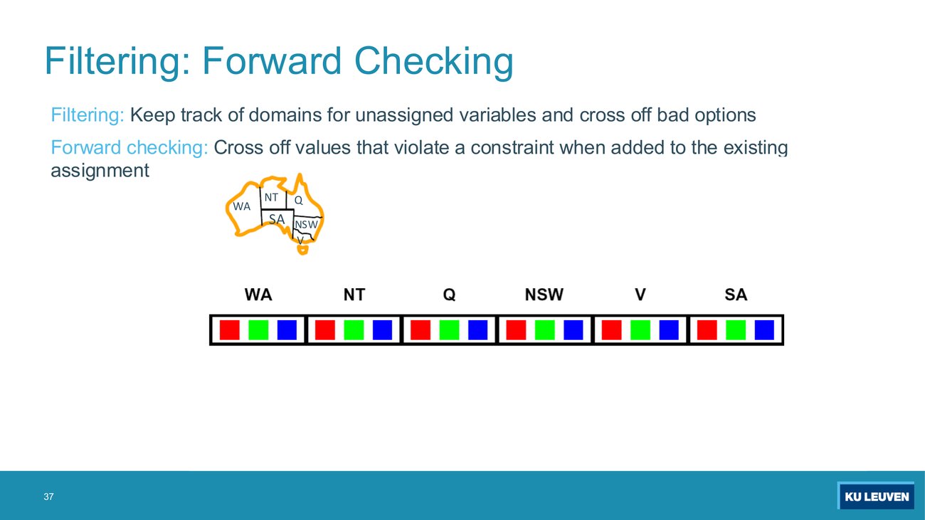
Animation build: this frame is the clean pre-filtering strip. All six strips still hold red, green and blue, nothing has been struck, and the map above them is an uncoloured outline, so the picture is the starting state before any assignment. Use it as the baseline; p.38 below carries the filtered version.
The next build assigns WA = red. Predict exactly which squares vanish from which strips, and which strips are untouched. Then state the rule in one sentence.
Red vanishes from NT and from SA. Q, NSW and V are untouched. Verified by executing forward checking on the Australia CSP: after WA = red the domains are WA={R}, NT={G,B}, Q={R,G,B}, NSW={R,G,B}, V={R,G,B}, SA={G,B}.
The rule: forward checking prunes the domains of the unassigned variables that are neighbours of the variable just assigned, and of nobody else. It removes exactly the values that conflict with the new assignment, and it stops there. It does not look at any other pair of variables, and it does not repeat.
Classic mistake (archetype A8): continuing to propagate after the first ring of neighbours. That is arc consistency, not forward checking, and it is the confusion the 2023 sample exam tests.
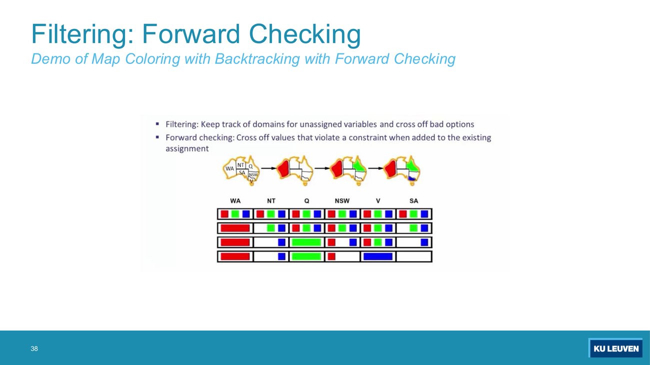
What this page actually is: not a later build of p.37. Page 38 is a separate slide titled "Filtering: Forward Checking" with the subtitle "Demo of Map Coloring with Backtracking with Forward Checking", and its body is an embedded screenshot of the original Berkeley slide. That screenshot contains the complete four-row forward-checking trace: the starting row plus one row after each of WA = red, Q = green and V = blue. Removed values are blank cells rather than struck-through glyphs, and an assigned variable is shown as one wide bar of its colour. Every row was checked against an executed run of forward checking and matches exactly.
Reproduce the four rows as a table, then fill the two cells left blank below. Assignment order WA = red, then Q = green, then V = blue.
| After | WA | NT | Q | NSW | V | SA |
|---|---|---|---|---|---|---|
| start | R G B | R G B | R G B | R G B | R G B | R G B |
| WA = red | R | G B | R G B | R G B | R G B | G B |
| Q = green | R | B | G | R B | R G B | B |
| V = blue | R | B | G | ? | B | ? |
Give the two missing entries and say what backtracking search does at that moment.
NSW = {R} and SA = { }, the empty set. Verified by executing forward checking: assigning V = blue prunes blue from its neighbours NSW and SA; NSW had {R,B} so it becomes {R}, and SA had only {B} so it becomes empty.
What happens next: forward checking has detected a wipeout. The current partial assignment {WA=red, Q=green, V=blue} cannot be extended to any solution, so backtracking undoes V = blue and tries the next value for V, without ever assigning NSW or SA. That is the entire benefit of filtering: the failure is found three variables early.
Notice also the row for Q = green: NT and SA are both reduced to {B}. Neither domain is empty, so forward checking says nothing is wrong. Deck p.39 puts its finger on exactly that row: "NT and SA cannot both be blue! Why didn't we detect this yet?" The answer is section 9.
2023 sample theory exam, MC 1.4, verbatim: the Part 6 slot, one true/false item per lecture
"In every step of the Forward Checking algorithm, it removes the values of all arcs that are not consistent."
How to answer it under pressure: the give-away words are "all arcs" and "every step". Forward checking never considers all arcs. Say to yourself: FC touches the ring of neighbours of one variable; AC-3 touches the whole graph and re-enqueues.
Constructed drillconstructed example: decide true or false for each. (a) "Forward checking can empty the domain of a variable that is not adjacent to the variable just assigned." (b) "After forward checking, every arc of the CSP is consistent." (c) "Arc consistency can be run before search starts as well as after each assignment."
(a) False. Only neighbours of the just-assigned variable are touched, so only a neighbour can be emptied. (b) False. The p.38 trace after Q = green leaves NT = {B} and SA = {B}, and the arc SA → NT is not consistent: SA's only value blue has no support in NT. (c) True, and it is printed on p.41: "Can be run as a preprocessor or after each assignment".
Exercise session 4, exercise 2, verbatim from FAI_Exercise_CSP.pdf p.3 (archetype A8)
"1. The 4-teachers problem. Four teachers, A, B, C and D have to give classes at the same time. To this end, 5 rooms are available, viz. rooms 1, 2, 3, 4 and 5. Teacher A doesn't want to teach in room 1. Teacher B doesn't want to teach in room 2. Teacher D wants to teach in a room whose number is greater or equal to 3, yet strictly less than the number of the room B is teaching in. Teacher C doesn't want to teach in a room adjacent to that of B (rooms with successive numbers are adjacent), nor in room 5. Obviously, we want to assign different rooms to different teachers.
2. Formulate the above constraint problem in terms of constraints over the variables A, B, C and D and the finite domain {1, 2, 3, 4, 5}, as in the 4-houses problem. Use Forward Checking to generate a solution to the problem by drawing the search tree (depth-first with forward checking between successive assignments by the backtracking algorithm). Clearly indicate at each step which elements are removed from the domains."
Constraints. Unary: A ≠ 1, B ≠ 2, C ≠ 5, D ≥ 3. Binary: D < B, |C − B| > 1, and all different (drawn as the pairwise arcs A≠B, A≠C, A≠D, B≠C, C≠D). Watch the wording of the D constraint: it is two constraints in one sentence, a unary lower bound and a binary comparison with B.
Domains after the unary step: A={2,3,4,5}, B={1,3,4,5}, C={1,2,3,4}, D={3,4,5}.
| Step | Assign | Domains after filtering | Removed, and by which constraint |
|---|---|---|---|
| 1 | A = 2 | A={2}, B={1,3,4,5}, C={1,3,4}, D={3,4,5} | 2 from C, by A ≠ C. B and D never held 2 in the first place. |
| 2a | B = 1 | A={2}, B={1}, C={3,4}, D={ } | 1 from C by |C − B| > 1, and all of {3,4,5} from D by D < B. Wipeout, fail. |
| 2b | B = 3 | A={2}, B={3}, C={1}, D={ } | 3 and 4 from C by |C − B| > 1, all of {3,4,5} from D by D < B. Wipeout, fail. |
| 2c | B = 4 | A={2}, B={4}, C={1}, D={3} | 3 and 4 from C by |C − B| > 1 and B ≠ C; 4 and 5 from D by D < B. Nothing empty, continue. |
| 3 | C = 1 | A={2}, B={4}, C={1}, D={3} | nothing left to remove. |
| 4 | D = 3 | A={2}, B={4}, C={1}, D={3} | Solution: A = 2, B = 4, C = 1, D = 3. |
Check it: A ≠ 1 (2), B ≠ 2 (4), C ≠ 5 (1), D ≥ 3 (3), D < B (3 < 4), |C − B| = 3 > 1, all four rooms distinct.
The problem has ten solutions, and the session-4 solution deck ends by listing all of them: (A,B,C,D) = (2,4,1,3), (2,5,1,3), (2,5,1,4), (2,5,3,4), (3,5,1,4), (3,5,2,4), (4,5,1,3), (4,5,2,3), (5,4,1,3), (5,4,2,3). Enumerated exhaustively and matched against that slide. Any one of them is a correct answer to "generate a solution"; which one you reach is decided entirely by your variable and value order, which is why section 11 revisits this same problem with MRV, degree and LCV and lands on (4,5,1,3) instead.
What earns the marks: the removed elements written at every node, struck through or listed, and the name of the constraint that removed each one. A node that just says "fail" earns nothing.
Deck p.39 makes the diagnosis: forward checking "propagates information from assigned to unassigned variables, but doesn't provide early detection for all failures", with the example "NT and SA cannot both be blue!", and the prescription: "Constraint propagation: reason from constraint to constraint".
Deck p.40 gives the definition everything rests on:
An arc X → Y is consistent iff for every x in the tail there is some y in the head which could be assigned without violating the constraint.
Two quantifiers, in that order, and they are the whole definition. Every value in the tail needs at least one partner in the head. A tail value with no partner is deleted. The slide adds the sentence that connects back to section 8: "Forward checking: enforcing consistency of arcs pointing to each new assignment".
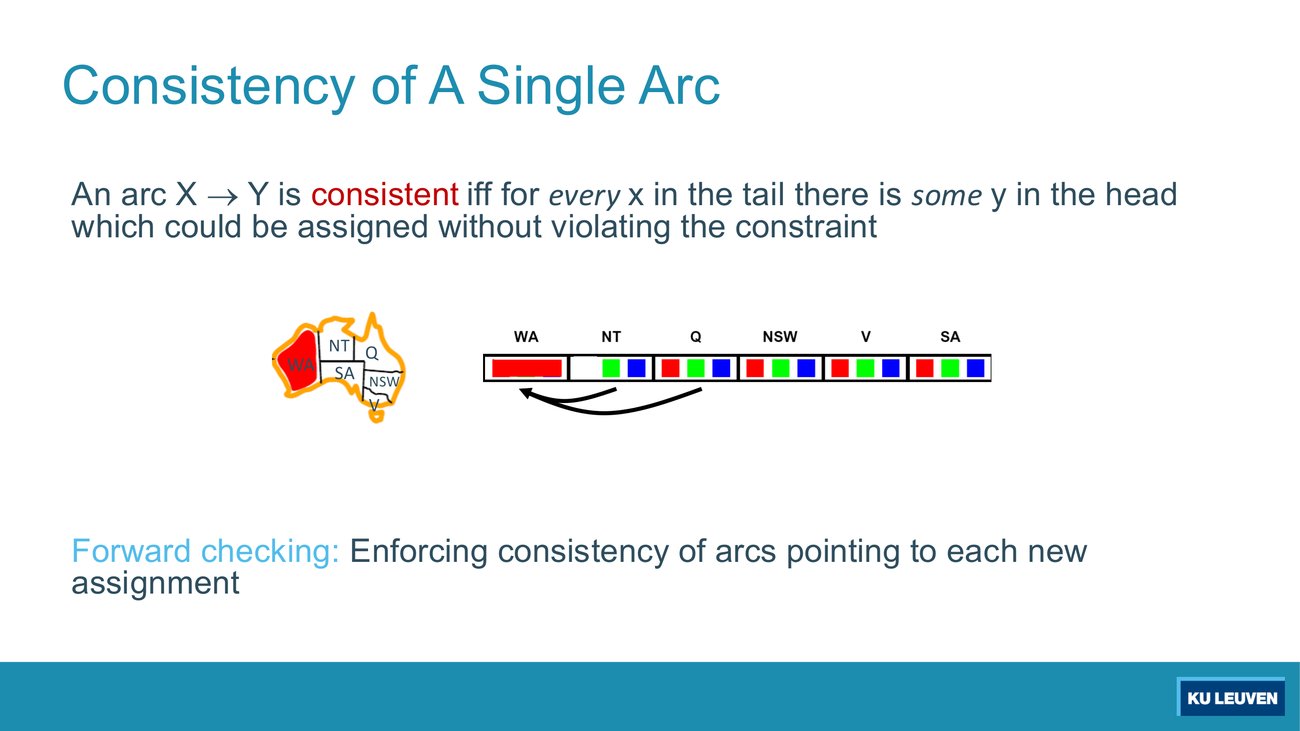
Take WA = {red} and NT = {red, green, blue}. Decide whether the arc WA → NT is consistent, and whether the arc NT → WA is consistent. If one of them fails, say exactly which value is deleted and from which variable.
WA → NT is consistent. The only tail value is red, and the head NT contains green, which differs from red. One partner is enough.
NT → WA is not consistent. The tail value red has no partner in WA = {red}, since the only head value equals it. So red is deleted from NT, the tail. NT becomes {green, blue}.
The direction is the trap. Deck p.41 prints a reminder box for exactly this: "Remember: Delete from the tail!". Arcs are directed, and each direction is a separate item of work; enforcing X → Y says nothing about Y → X.
as long as there is one value in the second domain that is consistent we keep this value.(Lecturer, T5), spoken while walking through the arc-consistency grid. This is the retention rule stated from the opposite side: you delete a tail value only when no head value supports it. Students who delete a tail value as soon as they find one conflicting head value are running a different, much too aggressive algorithm, and they will empty domains that are perfectly fine.
Deck p.41 then scales the definition to the whole problem: "a simple form of propagation makes sure all arcs are consistent", with three consequences printed underneath, all three examinable:
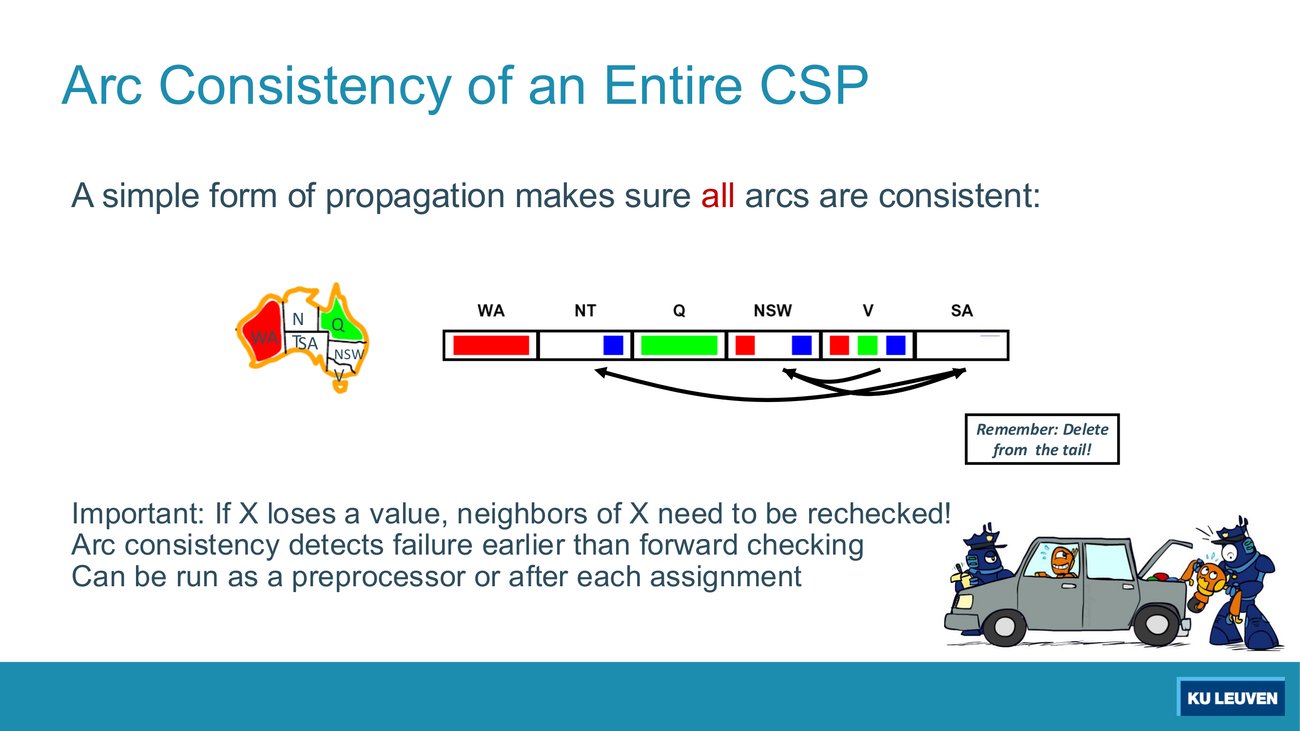
The grid shows the state after WA = red and Q = green: NT = {B}, NSW = {R,B}, V = {R,G,B}, and SA is empty. Name the single arc whose revision emptied SA, show the check that failed, and say what forward checking would have reported at this same moment.
The arc SA → NT. After forward checking on WA = red and Q = green, SA = {B} and NT = {B}. Revising SA → NT asks: does SA's value blue have a partner in NT that differs from it? NT holds only blue, so no. Blue is deleted from the tail, SA becomes empty, and AC-3 returns failure.
Forward checking would have reported nothing. Every domain is non-empty at that moment (NT={B}, SA={B}, NSW={R,B}, V={R,G,B}), so FC sees no problem and search continues, eventually assigning V and only then discovering the wipeout, as the p.38 trace shows. This is the precise content of "arc consistency detects failure earlier than forward checking", and both traces were executed to confirm it.
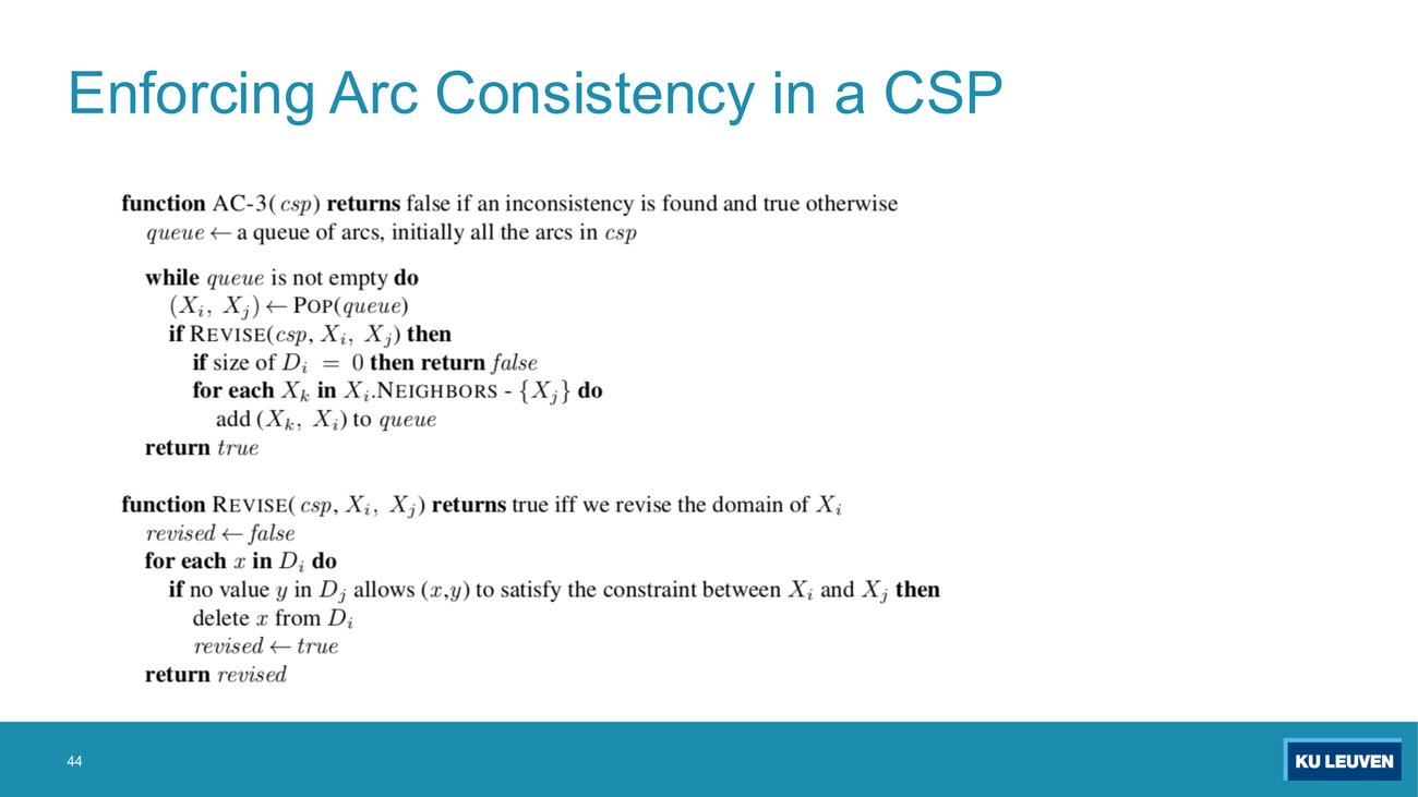
In the AC-3 pseudocode, after REVISE(csp, Xi, Xj) returns true and Di is non-empty, which arcs are added back to the queue? Write the exact form, and explain in one sentence why the arc that was just processed is excluded.
For each Xk in Xi.NEIGHBORS − {Xj}, add the arc (Xk, Xi) to the queue. Note the direction: the new arcs point into Xi, because Xi is the domain that just shrank, so it is the neighbours' support that may have disappeared.
Why Xj is excluded: the arc (Xj, Xi) cannot have become inconsistent as a result of this revision. Removing a value from Di can only destroy support for values in Dj, and the revision just performed removed only values of Di that had no support in Dj at all; re-checking (Xj, Xi) is provably wasted work here. Skipping it is an optimisation, not a change of result.
Classic mistakes (archetype A9): re-enqueueing (Xi, Xk) instead of (Xk, Xi), which propagates in the wrong direction; and forgetting to re-enqueue at all, which turns AC-3 into a single sweep and silently produces a weaker filter.
The exercise-session solutions write the queue as a literal list and append the re-enqueued arcs at the end, for example [(A,B),(B,A),(A,C),(C,A),(A,D),(D,A),(B,C),(C,B),(B,D),(D,B),(C,D),(D,C), (A,C),(B,C)] for the 4-houses problem. Do the same. Below is the same discipline on the Australia CSP after WA = red and Q = green, with the initial queue holding all 18 arcs (both directions of the nine constraints) in the order WA-NT, WA-SA, NT-SA, NT-Q, SA-Q, SA-NSW, SA-V, Q-NSW, NSW-V, and only the revisions that actually delete something shown.
| Arc popped | Deleted from tail | Domains after |
|---|---|---|
| NT → WA | R | WA=R, NT=GB, Q=G, NSW=RGB, V=RGB, SA=RGB |
| SA → WA | R | WA=R, NT=GB, Q=G, NSW=RGB, V=RGB, SA=GB |
| NT → Q | G | WA=R, NT=B, Q=G, NSW=RGB, V=RGB, SA=GB |
| SA → Q | G | WA=R, NT=B, Q=G, NSW=RGB, V=RGB, SA=B |
| NSW → SA | B | WA=R, NT=B, Q=G, NSW=RG, V=RGB, SA=B |
| V → SA | B | WA=R, NT=B, Q=G, NSW=RG, V=RG, SA=B |
| NSW → Q | G | WA=R, NT=B, Q=G, NSW=R, V=RG, SA=B |
| V → NSW | R | WA=R, NT=B, Q=G, NSW=R, V=G, SA=B |
| SA → NT | B | SA is empty, AC-3 returns false |
Two things to take from this table. First, exactly one of these nine revisions is the work of re-enqueueing, and it is the last one. Follow SA → NT through the run. It sits sixth in the initial queue, and when it is popped there both SA and NT still hold {green, blue}, so each of SA's two values has a partner in NT (green pairs with blue, blue with green) and nothing is deleted. The very next pop, NT → Q, cuts NT down to {blue}. That is the situation the slide's rule covers: NT has lost a value, so the arcs pointing into NT must be rechecked, and (SA, NT) is appended at the right-hand end of the queue. Its second visit, which happens only after all 18 initial arcs have been popped, is the revision that finally deletes blue from SA and empties it, and it is the only deleting revision in the whole run that comes from a re-enqueued arc. The other three late-firing arcs need no such story: NSW → SA, V → SA and V → NSW were still sitting in the initial queue, at positions 12, 14 and 18, when they fired. Stop after a single sweep of those 18 arcs and you end with WA={R}, NT={B}, Q={G}, NSW={R}, V={G}, SA={B}: every domain non-empty, no failure reported, and the contradiction missed. Both versions executed. Second, the failure surfaces on an arc between two unassigned variables, SA and NT, which is exactly the kind of interaction forward checking is structurally unable to see.
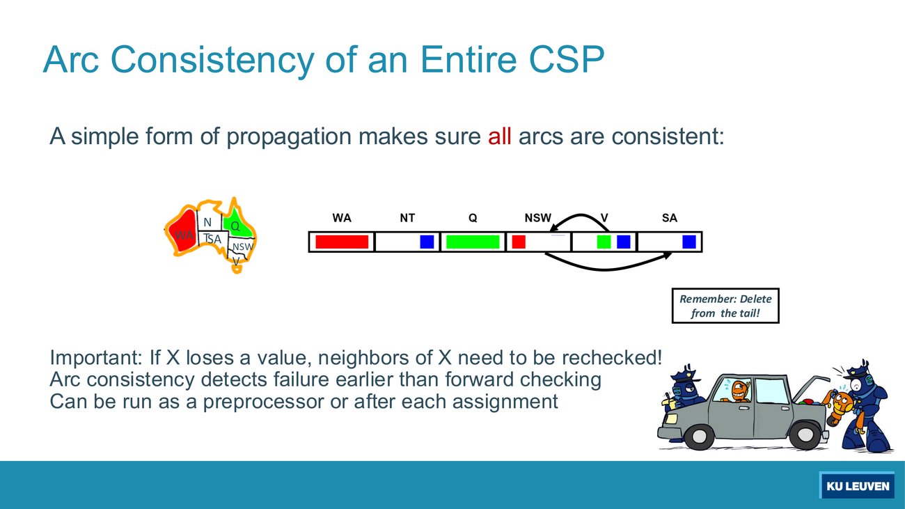
Animation build: pp.41 and 45 are the same slide, printed twice around the AC-3 pseudocode on p.44, and the PDF export froze a different animation frame each time. They start from the same state (forward checking after WA = red and Q = green) and show two different arcs having fired.
This frame shows NT = {B}, NSW = {R}, V = {G,B}, SA = {B}. Name the two revisions that produced it from the forward-checking state NT={B}, NSW={R,B}, V={R,G,B}, SA={B}. Then answer the real question: does the order in which AC-3 pops arcs change the final answer?
Revision 1, NSW → SA: NSW's value blue has no partner in SA = {B}, so blue is deleted and NSW becomes {R}. Revision 2, V → NSW: V's value red has no partner in NSW = {R}, so red is deleted and V becomes {G,B}. Both verified by executing REVISE on those domains.
No: provided the run is allowed to reach a fixpoint, the order does not change the outcome. With that condition in place, the set of values AC-3 removes is the same for every queue order, because removal is monotone: a value that has lost all its support can never regain support when other domains only shrink further. So the algorithm always reaches the same arc-consistent fixpoint, and order changes only the route and the amount of work.
The condition is not decoration. The pseudocode returns false the moment a domain empties, so a run that hits a wipeout stops before the fixpoint, and then which values have been deleted so far, and which variable is caught empty, do depend on the queue order. The trace table above is exactly such a run. What survives the order change is the verdict: from this same state, with the full 18-arc queue, AC-3 again terminates in failure, but the first empty domain is NT rather than SA, at the fifth pop, on the arc NT → SA. Both runs executed.
This is a useful thing to say in an exam when your trace differs from the model answer: if you ran to a fixpoint and the model answer deleted the same values in a different order, you are still right.
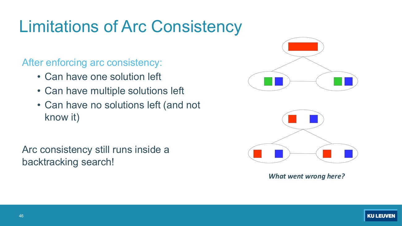
The slide asks "What went wrong here?" beside the lower graph, where all three mutually connected nodes hold {red, blue}. Check every arc of that graph for consistency, then say how many solutions it has. Explain why arc consistency cannot see the problem.
Every arc is consistent. Take any directed arc: the tail value red has the partner blue in the head, and the tail value blue has the partner red. Both quantifier conditions hold, so no value is ever deleted and AC-3 terminates reporting success with all domains intact.
There are zero solutions. Three mutually adjacent variables that must all differ need three distinct values, and only two are available. This is the third bullet on the slide: after enforcing arc consistency you "can have no solutions left (and not know it)".
Why it is invisible: arc consistency is 2-consistency, as p.48 makes explicit. It only ever inspects two variables at a time. The contradiction here is a genuine three-variable interaction and no pairwise check can expose it. The upper graph shows the opposite corner of the same slide: it is arc consistent and has two solutions, so a successful AC-3 run tells you neither that a solution exists nor that it is unique.
Consequence, printed on the slide and worth quoting back in an exam: "Arc consistency still runs inside a backtracking search!" Filtering is a pruning device, never a solver.
Exercise session 4, exercise 1, task 2, verbatim from FAI_Exercise_CSP.pdf p.2 (archetype A9)
"2. Now consider the following sets of partial assignments: {A = 1}, {A = 2, B = 2}, {A = 2, B = 3}, {A = 2, B = 3, C = 1}, {A = 2, B = 4}. Which of these can not be extended into a solution according to 1) forward checking, and 2) arc consistency"
Same 4-houses problem as section 7: unary C ≠ 3 and B ≠ 1, binary C > D, D = A − 1, |B − D| ≥ 2 and all different, starting domains A={1,2,3,4}, B={2,3,4}, C={1,2,4}, D={1,2,3,4}. Two filters, five assignments, ten decisions.
| Partial assignment | Forward checking | Arc consistency (AC-3) |
|---|---|---|
| {A = 1} | Rejected. A = 1 forces D = A − 1 = 0, so filtering the neighbour D empties its domain. | Rejected. A itself empties, on the arc A → D: no value of A has a partner d = A − 1 once D is down to {2,3,4}. C also loses 1. |
| {A = 2, B = 2} | Rejected before any filtering: A ≠ B is violated outright, which is the incremental goal test of section 7, not the filter. | Rejected. Revising A → B empties A: its only value 2 has no partner in B = {2}. |
| {A = 2, B = 3} | Survives. A={2}, B={3}, C={1,4}, D={1}, nothing empty. | Survives, and prunes further: the fixpoint is A={2}, B={3}, C={4}, D={1}, which is the unique extension. |
| {A = 2, B = 3, C = 1} | Rejected. C = 1 forces D < 1, so D empties. | Rejected. C empties on the arc C → D once D has been cut to {1}. |
| {A = 2, B = 4} | Survives. A={2}, B={4}, C={1}, D={1}. Both remaining domains hold exactly one value and neither is empty, so forward checking reports nothing. | Rejected. Revising C → D asks whether C's only value 1 has a partner d in D = {1} with c > d. It has none, 1 is deleted from the tail, and C is empty. |
The last row is the whole question. Forward checking leaves C = {1} and D = {1} side by side and cannot see that they contradict each other, because C and D are both unassigned and forward checking only ever compares an unassigned variable with the one just assigned. AC-3 compares them directly and dies on C > D. Score: forward checking rejects 3 of the 5, arc consistency rejects 4 of the 5, and no assignment is rejected by FC but accepted by AC-3, which is the ordering the question is built to demonstrate.
The queue, written as the solution deck writes it. For {A = 2, B = 3} the run is [(A,B),(B,A),(A,C),(C,A),(A,D),(D,A),(B,C),(C,B),(B,D),(D,B),(C,D),(D,C), (A,C),(B,C)]. The two arcs after the gap are the re-enqueued ones: popping (C,D) deletes 1 from C, so every arc pointing into C except (D,C) has to be rechecked, and both (A,C) and (B,C) had already been popped. Write the queue exactly like this, growing at the right-hand end, and the marker can follow the propagation.
What the question is really testing: that AC-3 rejects strictly more partial assignments than FC does, and that you can point at the arc responsible. An assignment rejected by FC is always rejected by AC-3; the interesting cases are the ones where FC says "ok" and AC-3 says "no".
Classic mistake: stopping after one sweep of the initial queue. If you never append an arc, you have not run AC-3.
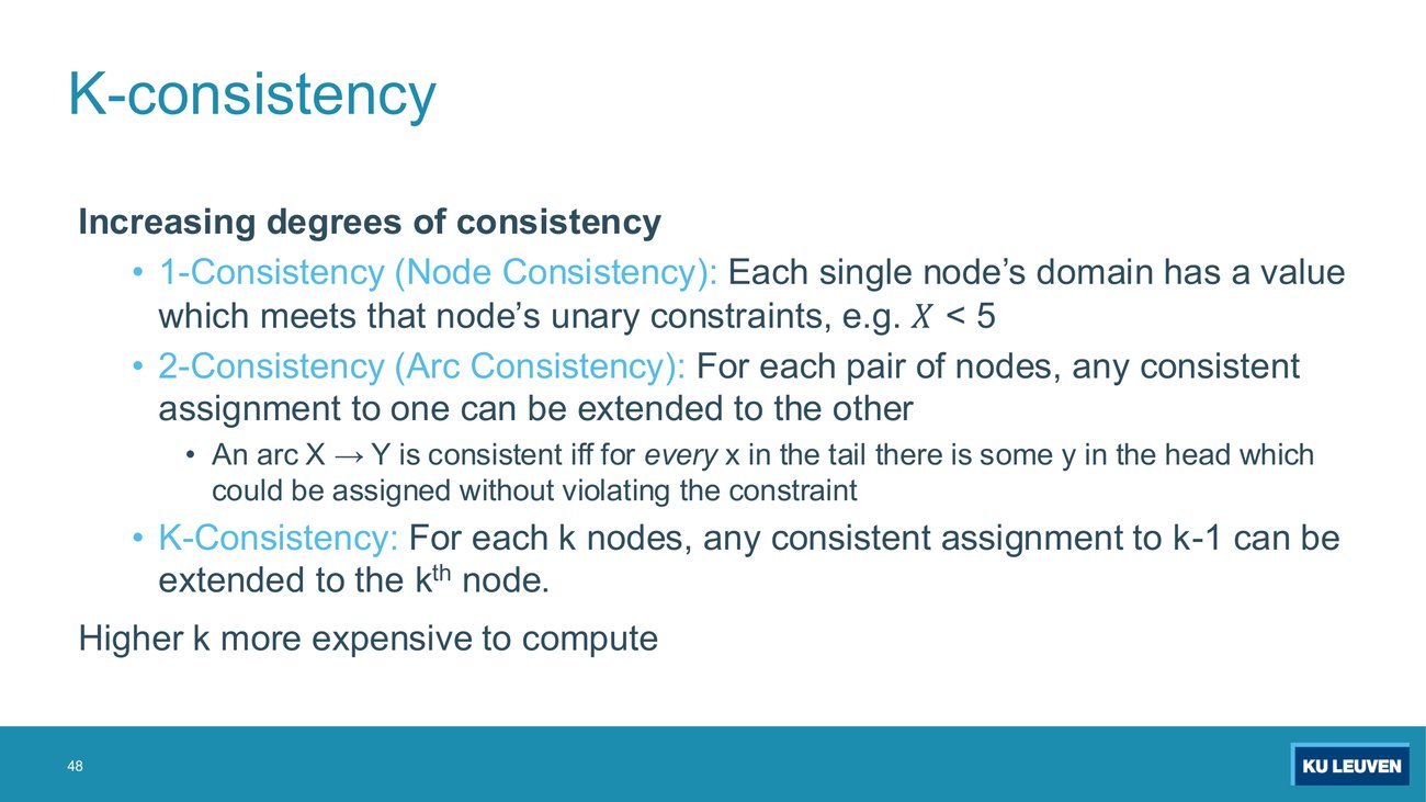
Using the ladder on this slide, name the lowest k whose enforcement would have detected the failure in the lower graph of p.46 (three mutually adjacent variables, domains {red, blue}, all-different). Show the check that fails. Then say what 1-consistency corresponds to in the exercise sessions.
k = 3. The slide's definition: "for each k nodes, any consistent assignment to k−1 can be extended to the kth node". Take the two-variable assignment X = red, Y = blue, which is consistent. Extending it to Z requires a value different from both red and blue, and the domain has none. So 3-consistency fails, and enforcing it would prune.
1-consistency, called node consistency on the slide, is the unary-constraint step. "Each single node's domain has a value which meets that node's unary constraints, e.g. X < 5". In exercise session 4 this is the very first thing you do: A ≠ 1, B ≠ 2, C ≠ 5, D ≥ 3 turn the domains {1,...,5} into A={2,3,4,5}, B={1,3,4,5}, C={1,2,3,4}, D={3,4,5} before any search happens.
The trade-off, printed on the slide: "Higher k more expensive to compute". Enforcing 3-consistency on a graph is far costlier than arc consistency, which is why AC-3 is the practical default and the one the course drills.
Deck p.50 sets up the two questions and the single principle behind both answers: "Variable ordering: which one to assign first? Value ordering: which value to try first? Principle: try to detect failures early on".
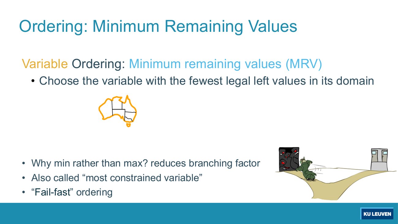
Animation build: the Australia outline on this frame carries no colours. The colouring appears in a later build. Basis for reading the intended state: the LCV slide p.54 of the same deck shows the same map with WA red and NT green as its starting picture, and the MRV argument on this slide is about the variable that is down to one value in exactly that situation.
Predict which two regions the later build colours in, and which variable minimum remaining values (MRV) then selects. Count the remaining values of every unassigned variable to justify the choice, and then explain the slide's own question, "Why min rather than max?".
WA becomes red and NT becomes green, and MRV selects SA. With those two assignments and filtering in force the remaining domains are: SA = {blue}, so 1 value; Q = {red, blue}, 2; NSW = {red, green, blue}, 3; V = {red, green, blue}, 3; T = {red, green, blue}, 3. Computed by running forward checking on WA = red then NT = green. SA is the unique minimum.
Why min: the slide answers it in four words, "reduces branching factor". The variable with the fewest values creates the fewest subtrees, and if it has zero values you discover the dead end immediately instead of after expanding the other variables. The slide also gives the alias, "most constrained variable", and the label "fail-fast ordering".
Classic mistake: taking the maximum. It is the natural reading of "most constrained", and it is wrong. See the lecturer's warning below.
it should be clear that you take the minimum instead of the maximum... the choice for the minimum number of values is intended to keep this branching factor as limited as possible.(Lecturer, T5), spoken over p.51, and also printed on the slide as "Why min rather than max? reduces branching factor". He says it out loud because "most constrained variable" sounds like it should mean "the one with the most options constrained away", and students then reach for the largest number in the row. The rule is: smallest domain wins.
it is also a so-called fail fast ordering because the idea is that you want to fail as quickly as possible.(Lecturer, T5), spoken here in the MRV, most-constrained-variable context; the phrase "fail-fast ordering" is printed on both p.51 and p.53. It is the same principle as p.35's "general idea: try to detect failure early on" and p.50's "principle: try to detect failures early on". Filtering and ordering are two implementations of one strategy: spend a little work now to avoid a lot of search later.
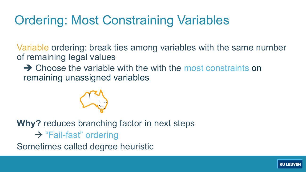
Animation build: the map on this frame is again an uncoloured outline; the illustration is completed in a later build.
The slide defines the tie-break: among variables with the same number of remaining legal values, choose the one with the most constraints on remaining unassigned variables (the deck's own wording, with its duplicated "with the", is quoted in the term box). Fill in the degree of each of the seven Australia variables at the very start of search, and name the variable this heuristic picks first.
| WA | NT | Q | NSW | V | SA | T |
|---|---|---|---|---|---|---|
| 2 | 3 | 3 | 3 | 2 | 5 | 0 |
SA, with degree 5. Degrees computed from the nine-constraint adjacency list. At the start every variable has three values, so MRV is a seven-way tie and the degree heuristic decides everything.
The words "remaining unassigned" are load-bearing. Degree is recomputed as search proceeds: a constraint to an already-assigned variable no longer branches anything, so it does not count. In the four-teachers drill below, the tie between A and C is not broken by degree, because at that point each of them has exactly one unassigned neighbour, namely the other.
Why it works: same reason as MRV, and the slide says so, "reduces branching factor in next steps", with the same "fail-fast ordering" label.
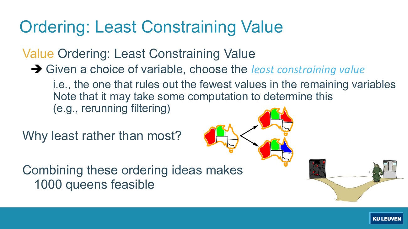
The state is WA = red, NT = green, and the variable being assigned is Q. Count, for each of the two branches drawn, how many values are left in SA afterwards. Then say which value the least constraining value (LCV) heuristic picks, and why that is the opposite instinct to MRV.
| Branch | SA after | Values left in SA |
|---|---|---|
| Q = red (upper map) | {blue} | 1 |
| Q = blue (lower map) | { } | 0 |
SA borders WA, NT and Q. With WA = red and NT = green, SA is already down to {blue}. Choosing Q = blue removes that last value and wipes SA out; choosing Q = red leaves it. So LCV picks red, the value that "rules out the fewest values in the remaining variables", in the slide's words.
Why the opposite instinct: variable ordering wants to fail fast, because you must eventually assign every variable, so a doomed subtree should die at once. Value ordering wants to succeed fast, because you only need one value per variable to work, so the most promising one should be tried first. The slide poses this as "Why least rather than most?" and it is a fair exam question. It also warns that LCV "may take some computation to determine this (e.g., rerunning filtering)", and claims the payoff: "combining these ordering ideas makes 1000 queens feasible".
This is the last exercise of session 4, "the 4 teachers problem revisited". Four teachers A, B, C, D are assigned to rooms 1 to 5, one room each. Unary constraints A ≠ 1, B ≠ 2, C ≠ 5, D ≥ 3 give the starting domains. Binary constraints: all different, D < B, and |C − B| > 1. Variable ordering MRV with the degree heuristic as tie-break, value ordering LCV, filter forward checking.
| Step | Domains | Choice and the counting that justifies it |
|---|---|---|
| 1 | A={2,3,4,5} B={1,3,4,5} C={1,2,3,4} D={3,4,5} |
MRV picks D (3 values, the unique minimum). LCV counts of values removed from the other three domains: D=3 removes 4 (A loses 3; B loses 1 and 3; C loses 3); D=4 removes 5; D=5 removes 5. Choose D = 3. |
| 2 | A={2,4,5} B={4,5} C={1,2,4} D=3 |
MRV picks B (2 values against 3 and 3). LCV: B=4 removes 2 (A loses 4, C loses 4); B=5 removes 2 (A loses 5, C loses 4). A genuine tie. The solution deck takes B = 5; B = 4 is equally defensible under LCV and also leads to solutions. |
| 3 | A={2,4} B=5 C={1,2} D=3 |
MRV ties A and C at 2 values each, and the degree tie-break does not separate them: the only unassigned pair is A and C, so each has degree 1. The solution deck picks A, marking the slide with a question mark. LCV on A: A=2 removes 1 (C loses 2); A=4 removes 0. Choose A = 4. |
| 4 | A=4, B=5 C={1,2}, D=3 |
C is the only variable left. Take C = 1. Final assignment A=4, B=5, C=1, D=3, reached with no backtracking at all. |
Sanity check the answer against the constraints: A ≠ 1 holds (4), B ≠ 2 holds (5), C ≠ 5 holds (1), D ≥ 3 holds (3), D < B holds (3 < 5), |C − B| = 4 > 1 holds, and all four rooms differ. The problem has ten solutions in total, enumerated exhaustively; this heuristic combination walks straight to one of them.
Exercise session 4, closing exercise, verbatim from FAI_Exercise_CSP.pdf p.4 (archetype A10)
"Four teachers, A, B, C and D have to give classes at the same time. To this end, 5 rooms are available, viz. rooms 1, 2, 3, 4 and 5. Teacher A doesn't want to teach in room 1. Teacher B doesn't want to teach in room 2. Teacher D wants to teach in a room whose number is greater or equal to 3, yet strictly less than the number of the room B is teaching in. Teacher C doesn't want to teach in a room adjacent to that of B (rooms with successive numbers are adjacent), nor in room 5. Obviously, we want to assign different rooms to different teachers. Find a solution using backtracking. Use Forward checking as filter, and minimum remaining values as variable ordering (as tie breaker consider most constraining variable (i.e. degree heuristic)). As value ordering, employ least constraining value."
The worked drill directly above this box is the answer in full, with every LCV count written out. In short: MRV picks D (3 values), LCV then compares D = 3 removing 4 values against D = 4 and D = 5 removing 5 each, so D = 3; MRV picks B (2 values), LCV ties at 2 removals for both, the solution deck takes B = 5; MRV ties A and C at 2 values and the degree tie-break does not separate them either, the deck picks A, and LCV gives A = 4 because it removes nothing; C = 1 is then forced in spirit and taken. Final assignment A = 4, B = 5, C = 1, D = 3, reached with no backtracking. Every count was reproduced by executing forward checking, and the assignment matches the session-4 solution deck, which writes its counts on the slide as "D=3 eliminates: A:{3}, B:{1,3}, C:{3} # 4".
Note the two genuine ties at steps 2 and 3. They are in the published solution too, and the deck marks the second one with its own question mark. A tie is not a mistake in your working; failing to say how you broke it is.
Same problem, different answer. The plain forward-checking run of archetype A8, with the alphabetical order A, B, C, D and ascending values, reaches (2,4,1,3) instead. Both are among the ten solutions. The heuristics do not change what a solution is, only how fast you fall into one.
Order of application, in this order every time: pick the variable by MRV, break ties by degree over the unassigned neighbours, then order that variable's values by LCV.
Classic mistake: asserting instead of counting. LCV requires you to write down, for each candidate value, how many values it removes from each neighbour, and to total them. Students name a value that "looks less restrictive" and lose the marks that were allocated to the counting. Write the counts next to the branch, as the solution deck does with "D=3 eliminates: A:{3}, B:{1,3}, C:{3} # 4".
Second classic mistake: assuming the heuristics always break the tie. Step 2 and step 3 above are real ties that neither LCV nor degree resolves. If that happens, state your tie-break rule (for example lowest value, or alphabetical) and apply it consistently. A marker cannot fault a stated rule.
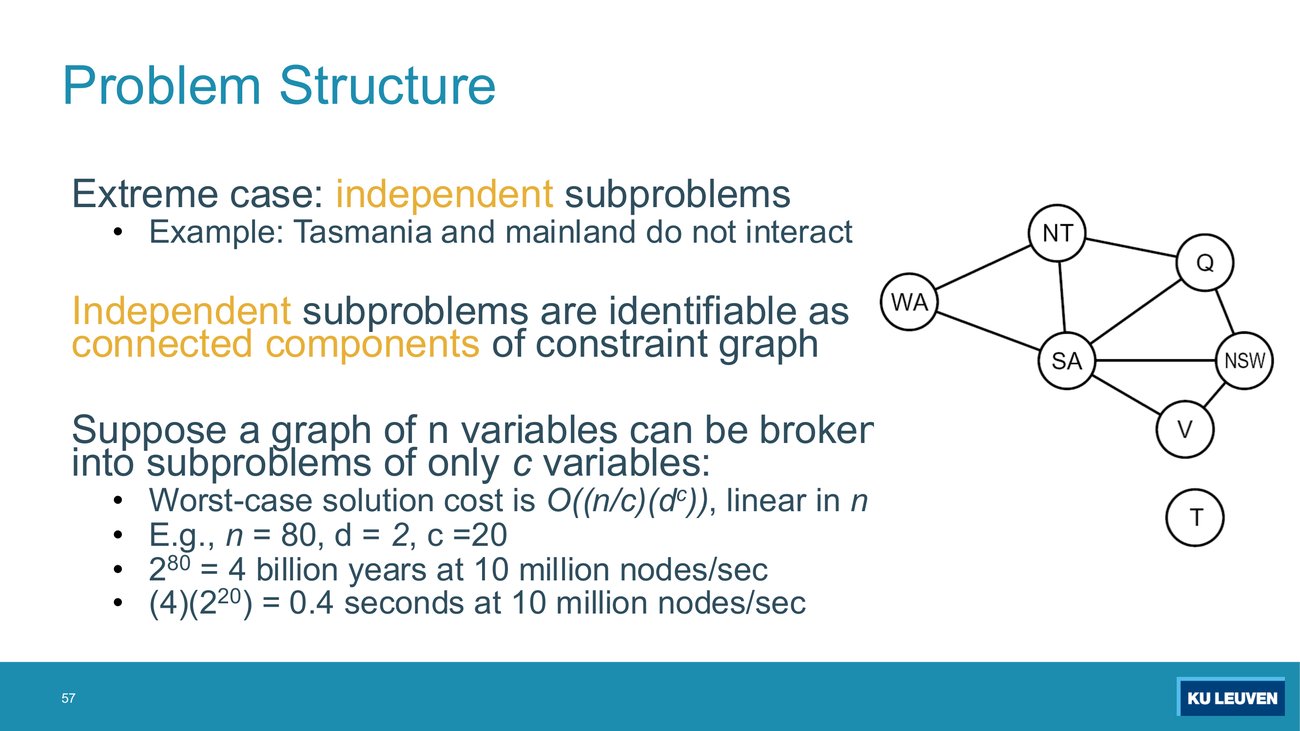
The slide states that if n variables split into subproblems of c variables each, the worst-case cost is O((n/c)(dc)), "linear in n", and then gives n = 80, d = 2, c = 20 with two numbers. Check both: 280 at 10 million nodes per second, and (4)(220) at the same rate. State the graph-theoretic recipe for finding the subproblems.
280 = 1.209 × 1024 nodes. Divided by 107 nodes per second that is 1.209 × 10¹⁷ seconds, which is 3.83 × 10⁹ years, so the slide's "4 billion years" is right. (4)(220) = 4,194,304 nodes, divided by 107 is 0.419 seconds, so "0.4 seconds" is right. Both computed.
The recipe, printed on the slide: "Independent subproblems are identifiable as connected components of constraint graph". Tasmania is its own component, so its three colour choices multiply the mainland's solutions rather than interacting with them. That is why the whole CSP has 18 solutions and the mainland alone has 6.
The factor here is 4 × 220 against 280, a ratio of about 3 × 10¹⁷. The lesson is that structure is not a micro-optimisation; it changes the exponent.
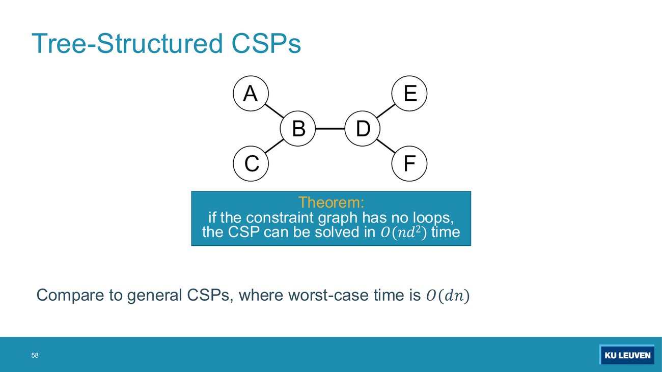
The theorem reads: "if the constraint graph has no loops, the CSP can be solved in O(nd2) time", compared with O(dn) in general. Explain where the n, the d2 and the absence of an exponent come from. What breaks if the graph has one cycle?
The n: a tree on n nodes has exactly n − 1 edges, so the backward pass performs n − 1 arc revisions and the forward pass makes n assignments. Both are linear in n. The d2: one call to Make-Arc-Consistent on an arc scans each of up to d values in the tail and, for each, up to d values in the head, so d × d work per arc.
Why there is no exponent: because no backtracking ever happens. Once every parent-to-child arc is consistent, section 12 shows that the forward pass can always find a value, so the algorithm never has to undo a choice. That is the whole content of the theorem: tree structure converts search into propagation.
One cycle breaks it, because a variable then has two paths of influence and making each arc consistent separately no longer guarantees a globally consistent choice. The p.46 triangle is the smallest example. The repair is cutset conditioning, below.
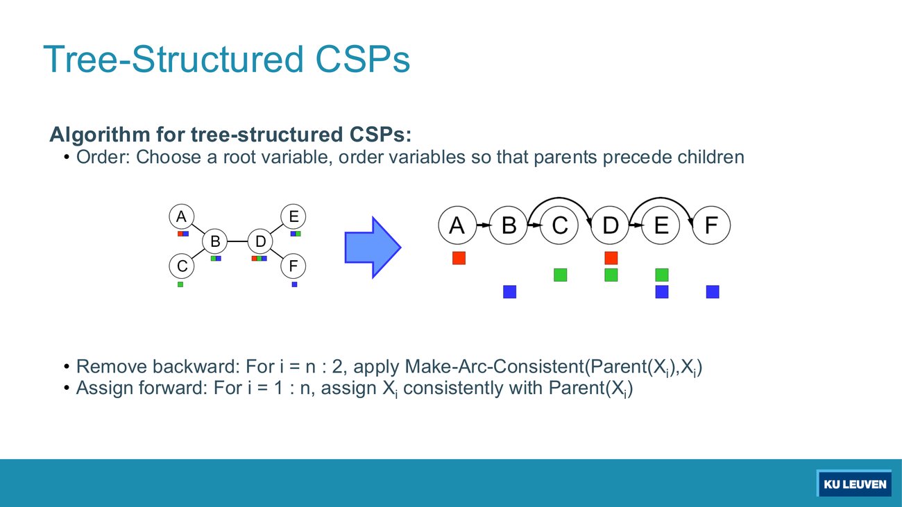
Left of the arrow, the tree is A−B, B−C, B−D, D−E, D−F, with domains A={R,B}, B={G,B}, C={G}, D={R,G,B}, E={G,B}, F={B} and the all-different constraint on every edge. Right of the arrow is the linearized chain after the backward pass. Fill in which values were removed from which variable, and by which arc, in the order the algorithm performs them.
| i | Arc revised | Deleted | Domain after |
|---|---|---|---|
| 6 | D → F | B from D | D = {R,G} |
| 5 | D → E | nothing | D = {R,G} |
| 4 | B → D | nothing | B = {G,B} |
| 3 | B → C | G from B | B = {B} |
| 2 | A → B | B from A | A = {R} |
Final domains A={R}, B={B}, C={G}, D={R,G}, E={G,B}, F={B}, which is exactly the right-hand strip on the slide. Verified by executing the backward pass.
Two things to notice. First, deletions happen in the parent, the tail of the arc, never in the child. Second, the order matters in one direction only: because i runs from n down to 2, every child is finished before its parent is revised, so a single sweep suffices and nothing needs re-enqueueing. The deletion of G from B at i = 3 is what later forces B out of A's domain at i = 2; had you processed the arcs in the other order you would have needed a second pass.
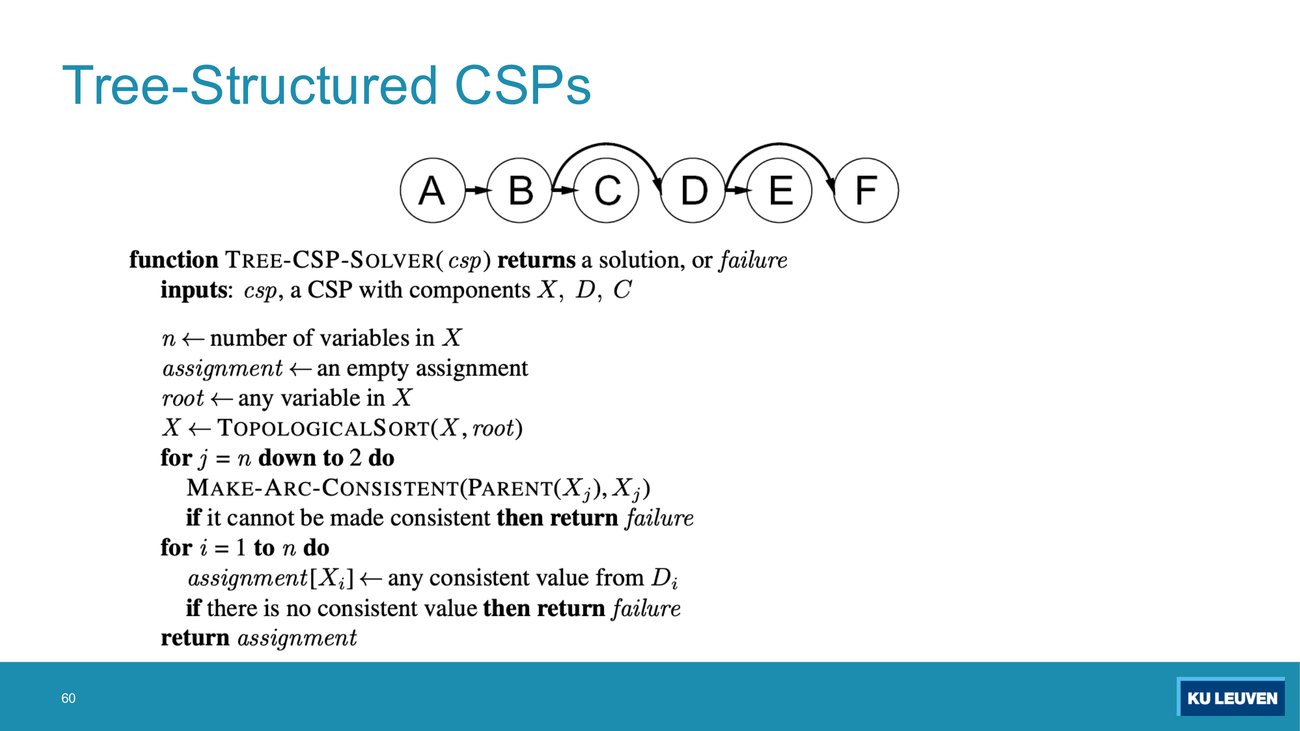
The pseudocode's second loop is "for i = 1 to n, assignment[Xi] ← any consistent value from Di". Run that forward pass on the reduced domains from the previous task, taking the first listed value each time in the order red, green, blue. Give the complete assignment, and say why the pseudocode's "if there is no consistent value then return failure" line can never fire here.
A = red (the only value). B = blue (only value, and it differs from red). C = green (only value, differs from B = blue). D: parent B = blue, and D = {R,G}, so red is consistent, D = red. E: parent D = red, E = {G,B}, so E = green. F: parent D = red, F = {B}, so F = blue. Verified by executing the forward pass. Choosing D = green instead would also work and would give a second solution.
Why failure cannot occur: the backward pass made every arc Parent(Xi) → Xi consistent, which means that for every surviving value of the parent there is at least one value of the child that fits. The forward pass assigns parents before children, so when you reach a child its parent already holds a surviving value, and a partner is therefore guaranteed. This is the property that removes backtracking, and the exercise-session slide states it in the same words: "given that the domains after enforcing consistency are non-empty, a solution is guaranteed".
Exercise session 4, exercise 3, verbatim from FAI_Exercise_CSP.pdf pp.3 and 4 (archetype A11)
"Brad, Daniel, Freddy, Jana, Kyle, Mike, and Nicholas are going on a team building event. During a brainstorming session they came up with the following events and associated event start times: 1. Kayaking (07:00) 2. Sightseeing (08:00) 3. Playing boardgames (8:15) 4. Hiking (09:00) 5. Bar hopping (20:00) 6. Movie night (22:00). Everyone has to participate in one event (but an event can obviously have multiple team members assigned to it, or possibly even none). There are however quite a few requirements that need to hold in order to reach a satisfactory activity assignment.
Questions: 1. Specify the constraint graph for this problem. Indicate the domain of each variable after applying unary constraints. 2. Find a solution by applying the algorithm for solving tree-structured CSPs (the two-pass algorithm). Start from a linearized version of the constraint graph by choosing K as the root."
First move, and the published solution says so on its own slide: replace the six activities by the numbers 1 to 6 in start-time order, so that every "starts before" requirement becomes an arithmetic < or >. 1 = kayaking (07:00), 2 = sightseeing (08:00), 3 = board games (08:15), 4 = hiking (09:00), 5 = bar hopping (20:00), 6 = movie night (22:00).
Question 1a, the constraint graph. Six binary constraints over seven variables: D ≠ J, M > N, J > N, D > K, N ≠ B, D < F. Seven nodes and six edges with the graph connected means no cycle, so it is a tree and the p.58 theorem applies. Everything else in the list is unary and belongs in the domains, not in the graph.
Question 1b, domains after the unary constraints: K={1,2,3}, M={1,3,5}, N={1,2,3,4,5} (no movie night), B={5}, F={1,2,3}, D={1,2,3,4,6} (no bar hopping), J={1,2,3,4,5,6}, which is untouched because Jana has no unary requirement.
Question 2, linearization rooted at K: K, D, F, J, N, B, M, with parent arcs K to D, D to F, D to J, J to N, N to B and N to M. Parents precede children, which is the only property the order has to have.
| i | Arc revised | Deleted from the parent | Parent domain after |
|---|---|---|---|
| 7 | N → M | 5, since M holds nothing above 5 | N = {1,2,3,4} |
| 6 | N → B | nothing | N = {1,2,3,4} |
| 5 | J → N | 1, since no value of N is below 1 | J = {2,3,4,5,6} |
| 4 | D → J | nothing | D = {1,2,3,4,6} |
| 3 | D → F | 3, 4 and 6, since F stops at 3 | D = {1,2} |
| 2 | K → D | 2 and 3, since D stops at 2 | K = {1} |
Domains after the backward pass: K={1}, D={1,2}, F={1,2,3}, J={2,...,6}, N={1,...,4}, B={5}, M={1,3,5}. Nothing is empty, so by the property on the exercise slide, "given that the domains after enforcing consistency are non-empty, a solution is guaranteed".
| Variable | Parent and its value | Value chosen | Activity |
|---|---|---|---|
| K | root | 1 | kayaking |
| D | K = 1, needs D > 1 | 2 | sightseeing |
| F | D = 2, needs F > 2 | 3 | board games |
| J | D = 2, needs J ≠ 2 | 3 | board games |
| N | J = 3, needs N < 3 | 1 | kayaking |
| B | N = 1, needs B ≠ 1 | 5 | bar hopping |
| M | N = 1, needs M > 1 | 3 | board games |
Final answer: Kyle kayaking, Daniel sightseeing, Freddy board games, Jana board games, Nicholas kayaking, Brad bar hopping, Mike board games. Both passes were executed independently and match the solution deck. Note that several people share an activity, which the question explicitly allows ("an event can obviously have multiple team members assigned to it"); a student who assumes the activities must all differ has added a constraint that is not there.
Order of operations, and each step earns marks: (1) apply the unary constraints to shrink domains, (2) draw the constraint graph and check it really is a tree, (3) linearize from the given root so that parents precede children, (4) backward pass right to left, revising Parent → Child and deleting from the parent, (5) forward pass left to right, choosing any consistent value.
Classic mistakes: skipping the unary step, so every later domain is wrong; deleting from the child instead of the parent in the backward pass; and running the two-pass algorithm on a graph that is not actually a tree, which is not merely inaccurate, it is unsound.
Deck p.61 states the general repair for graphs that are nearly trees. Conditioning: "instantiate a variable, prune its neighbors' domains". Cutset conditioning: "instantiate (in all ways) a set of variables such that the remaining constraint graph is a tree".
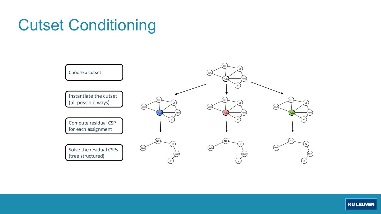
The slide's four steps are: choose a cutset, instantiate the cutset in all possible ways, compute the residual CSP for each assignment, solve the residual CSPs (tree structured). Here the cutset is {SA} and there are three residual problems. Write the total cost as a formula in n, d and the cutset size c, and name the trap in the phrase "in all possible ways".
Cost: O(dc · (n − c) d2). You enumerate every assignment of the c cutset variables, which is dc possibilities, and for each you solve a tree on the remaining n − c variables in O((n − c) d2) by the two-pass algorithm. Here c = 1 and d = 3, so three residual trees.
The trap: the cost is exponential in the cutset size, not in n. Cutset conditioning is a win only when a small set of variables destroys every cycle. If the cutset had 20 variables and d = 3, you would be enumerating 320 residual problems and the tree structure would buy you nothing. Notice also that removing SA from the Australia graph leaves the path WA−NT−Q−NSW−V together with the isolated node T, that is, a forest rather than a single tree; it is still loop-free, so the p.58 theorem still applies, component by component. That is why one cutset variable suffices in this example. Note too that finding a minimum cutset is itself a hard problem.
A second trap: "compute residual CSP" is not just deleting the node. You must also prune the neighbours' domains against the value you gave the cutset variable, which is the conditioning step defined on p.61.
Deck p.63 states the phenomenon and the fix. In map colouring with three colours "there are 3! = 6 symmetric solutions. These can be obtained by simply permuting the colors", and the search can be shrunk "by using symmetry breaking constraints", printed as "WA < SA, SA < Q, WA < Q (thus WA < SA < QA)". The lecture emphasised this slide, including the point that a single solution generates the other five by permutation.
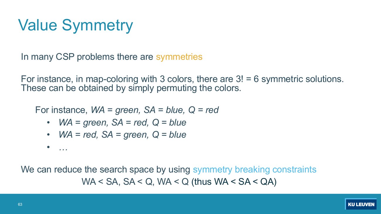
The six mainland regions have exactly six solutions. First, describe their structure: which regions always share a colour? Second, apply the slide's three constraints WA < SA, SA < Q, WA < Q literally to those six solutions and count how many survive. The answer is not five and not one.
Structure. Enumerating all 36 = 729 colourings of WA, NT, Q, NSW, V, SA gives exactly 6 that satisfy the nine constraints, and every one of them has the same shape: WA = Q = V take one colour, NT = NSW take a second, and SA takes the third. The six solutions are precisely the 3! = 6 ways of dealing three colours to those three groups, which is exactly the symmetry claim on the slide, confirmed by enumeration.
Applying the three constraints literally leaves zero solutions. WA and Q are never different, so WA < Q can never hold. Forced by the graph: WA, NT and SA form a triangle and so use all three colours, and Q must differ from both NT and SA, which leaves it only WA's colour.
The lesson, which is the examinable one: symmetry breaking is sound only if the added constraints keep at least one member of every symmetry class. A strict total order imposed on three variables that cannot all be pairwise different is too strong, and it turns a satisfiable problem into an unsatisfiable one. The correct version of the idea for this map is an order on variables that can differ, for example WA < SA and SA < NT, which is satisfied by exactly one of the six solutions. The principle on the slide is right; the specific triple is a generic illustration and does not survive contact with this particular graph.
Deck p.65 extends the framework: "most real-world problems involve an optimisation problem", with variables (finite domain), constraints, and an objective function. The abbreviation is printed on the slide: COP = Constraint Optimisation Problem. This is the same soft-constraint idea that p.22 deferred.
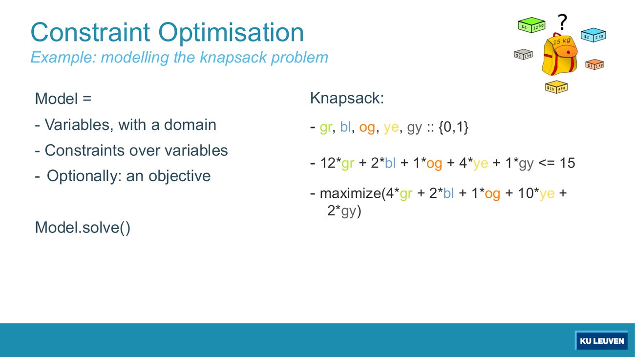
The model is: five boolean variables gr, bl, og, ye, gy; the constraint 12·gr + 2·bl + 1·og + 4·ye + 1·gy ≤ 15; the objective maximize(4·gr + 2·bl + 1·og + 10·ye + 2·gy). Solve it by hand. Give the optimal selection, its weight and its objective value.
Take bl, og, ye and gy; leave gr out. Weight 2+1+4+1 = 8, objective 2+1+10+2 = 15. Verified by enumerating all 32 subsets.
The reasoning by hand: gr costs 12 of the 15 units of capacity and returns only 4. Dropping it frees enough room for everything else, whose total weight is only 8. Taking gr forces you to leave out at least ye (weight 4), and the best you can then reach is 4 + 2 + 2 = 8. So the constraint is not even tight at the optimum, which is a good reminder that a capacity constraint being slack is not evidence of a modelling error.
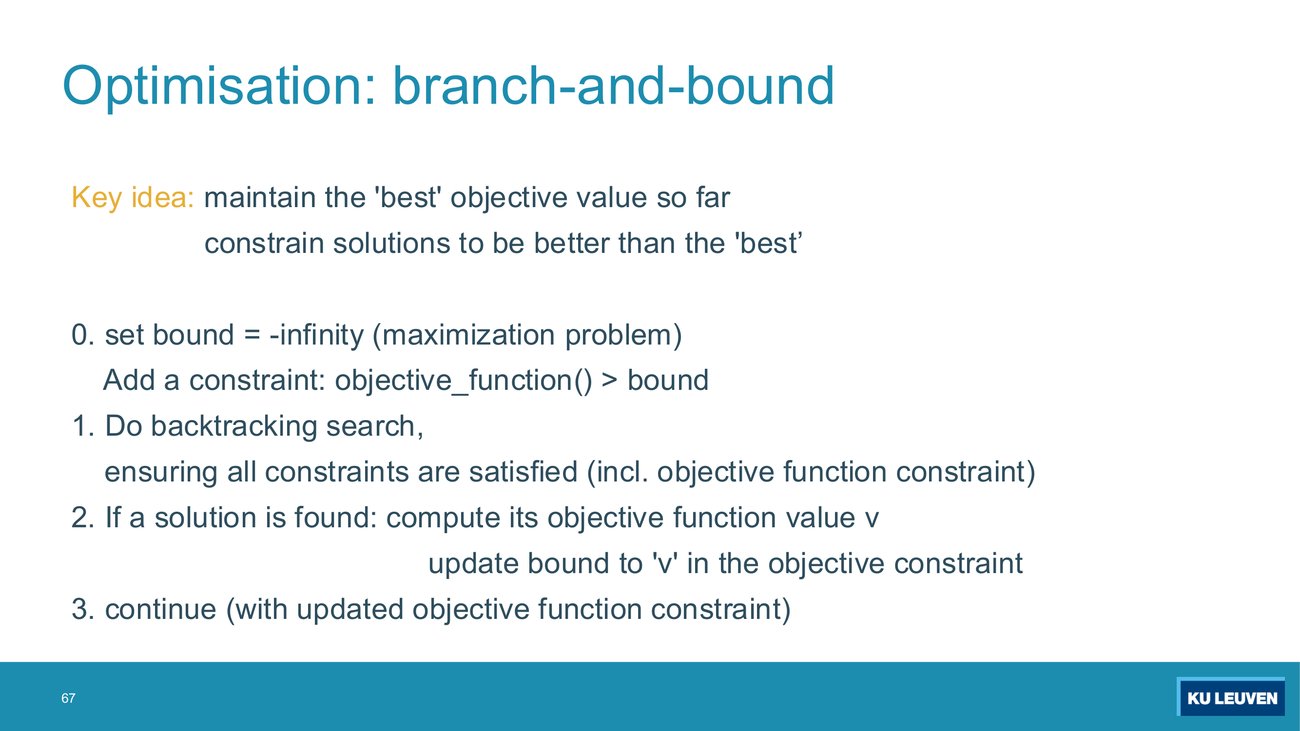
Suppose the search finds its first feasible knapsack selection with objective value 8. Predict exactly what changes in the problem being searched, what happens to the parts of the tree already explored, and how you know when the last solution found is optimal.
What changes: the constraint objective_function() > bound is rewritten with bound = 8, so every later node must promise more than 8 or be rejected. Nothing else about the problem changes; the search continues from where it was, not from the root.
Already-explored parts stay explored. The tightened constraint only prunes what comes next. This is why the algorithm is described on the slide as "continue (with updated objective function constraint)" rather than restart.
Optimality: when the search finishes and no further solution satisfies the tightened constraint, the last solution found is optimal, because any better one would have satisfied it. Note the constraint is a strict inequality, so a second solution of exactly equal value is also rejected; the procedure returns one optimum, not all of them.
I won't go into uh much more detail on this.(Lecturer, T5), spoken about branch-and-bound on p.67. This is an explicit limitation, so you can rely on it: the four numbered steps on the slide are the required depth. You should be able to state the key idea (keep the best objective value so far and constrain solutions to beat it), explain why that prunes, and say that optimisation sits on top of the same backtracking search. You are not expected to produce bounding functions or a branch-and-bound tree.
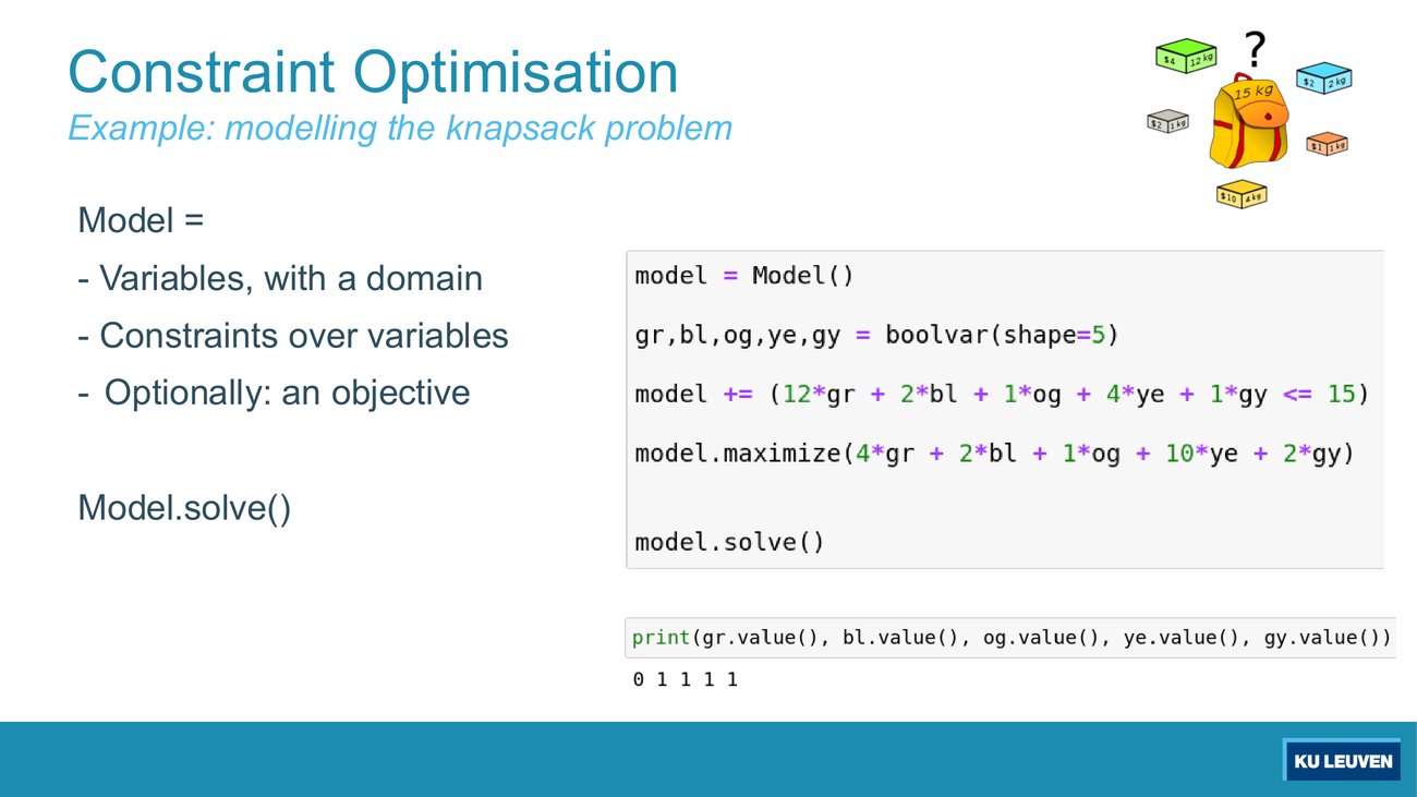
The code declares gr,bl,og,ye,gy = boolvar(shape=5), adds the weight constraint, calls model.maximize(...) and model.solve(), then prints 0 1 1 1 1. Decode that output into a selection, a weight and an objective value, and check it against your hand answer from p.66. Then map the three lines of the model onto the three bullets of the "Model =" box.
0 1 1 1 1 means gr = 0, bl = og = ye = gy = 1: leave the green item, take the other four. Weight 8, objective 15. Identical to the hand computation, as it should be.
Mapping: boolvar(shape=5) is "variables, with a domain"; model += (...≤15) is "constraints over variables"; model.maximize(...) is "optionally: an objective"; model.solve() is the solver call. That four-line shape is the whole point of the slide: modelling and solving are separated, so you declare what a solution is and the library decides how to find it. That separation is the same one that Part 10 exploits with SAT solvers.
Deck p.70 presents CPMpy as "a modern C(S)P library" and links three worked example notebooks: graph colouring of Australia, N-queens up to N = 1000, and a folder of industrial examples with visualisations on toy data. Deck p.71 is titled "Integrated constraint solving" and prints a Sudoku Assistant app image, a phone screenshot and the address https://visualsudoku.cs.kuleuven.be. Reading "integrated" as a machine-learning front end feeding a constraint solver is an inference from the title and the camera screenshot, not something the slide spells out. Both pages are tooling, offered in the same "try it yourself" spirit as the six Carnegie Mellon demo links printed earlier in the deck (pp.29, 33, 42, 43, 52, 55). Working through the notebooks is a good way to see the ordering heuristics pay off at N = 1000, which is a scale no hand trace reaches. Nothing you have to execute by hand depends on the library: the deck's own summary on p.72 lists only ordering, filtering and structure, and exercise session 4 asks for pen-and-paper traces throughout, with no code.
Deck p.72 compresses the Part into six lines: CSPs are a special kind of search problem, states are partial assignments, the goal test is defined by constraints, the basic solution is backtracking search, and the speed-ups are ordering, filtering and structure. If you can expand each of those six lines into a paragraph with an example, you have the theory half.
the slides and the material for the exercise sessions uh are the main source of reference. So that's the basis of what you need to know uh for the evaluation.(Lecturer, T1), also printed on the Part 1 slides. For this Part that means the 73 deck pages and exercise session 4, and nothing beyond them is required.
| Term | Precise definition | Plain paraphrase | Exam phrasing |
|---|---|---|---|
| CSP | A search problem whose state is defined by variables Xi with values from a domain D, and whose goal test is a set of constraints on subsets of those variables (p.11). | Fill in every variable so that no rule is broken. | "CSPs are specialized for identification problems" (p.10) |
| Identification vs planning | In an identification problem only the final assignment matters, not the path; in a planning problem the path is the answer (p.10). | The destination, not the journey. | "The goal itself is important, not the path" (p.10) |
| Constraint graph | Nodes are variables, arcs are constraints; binary CSPs give an ordinary graph, higher-order constraints need a hypergraph with one node per constraint (pp.16, 17). | A picture of which variables can affect which. | "nodes are variables, arcs show constraints" (p.16) |
| Backtracking search | Depth-first search plus two improvements: assign one variable at a time in a fixed order, and check constraints incrementally as values are added (p.31). | DFS that refuses a value the moment it clashes with what is already assigned. | "Backtracking = DFS + value consistency + fail-on-violation" (p.34) |
| Forward checking (FC) | After assigning a variable, delete from the domains of its unassigned neighbours every value that conflicts with the new assignment; no further propagation (p.37). Equivalently, enforce consistency of the arcs pointing at the new assignment (p.40). | Prune one ring of neighbours, once. | "In every step of the Forward Checking algorithm, it removes the values of all arcs that are not consistent" (sample theory MC 1.4, False) |
| Arc consistency, tail and head | In the arc X → Y, X is the tail and Y the head. The arc is consistent iff for every value in the tail there is some value in the head satisfying the constraint; unsupported values are deleted from the tail only. The CSP is arc consistent when all arcs are (pp.40, 41). | Every value of X needs at least one partner in Y, or it goes; the deletion happens at the arrow's start. | "Remember: Delete from the tail!" (pp.41, 45); "as long as there is one value in the second domain that is consistent we keep this value" (Lecturer, T5) |
| AC-3 | Queue-driven arc consistency: pop an arc, REVISE the tail, and on any deletion push (Xk, Xi) for every neighbour Xk of Xi except Xj; return false if a domain empties (p.44). | Keep revising arcs until nothing changes, re-queuing the neighbours of any domain that shrank. | "If X loses a value, neighbors of X need to be rechecked!" (pp.41, 45) |
| Node consistency and k-consistency | For any k nodes, every consistent assignment to k−1 of them extends to the kth. k = 1 is node consistency, that is, applying the unary constraints (which p.22 calls "equivalent to reducing domains"); k = 2 is arc consistency; higher k costs more (pp.22, 48). | Look at k variables at a time instead of two; k = 1 is just crossing the forbidden values out up front. | "Indicate the domain of each variable after applying unary constraints" (exercise session 4); "Higher k more expensive to compute" (p.48) |
| MRV | Variable ordering: choose the variable with the fewest legal values left; also called most constrained variable, a fail-fast ordering (p.51). | Assign the most cornered variable first. | "Why min rather than max? reduces branching factor" (p.51) |
| Degree heuristic | Tie-break among equal-MRV variables by choosing the one with the most constraints on the remaining unassigned variables (p.53). | Of the equally cornered, take the one that squeezes the most others. | "Choose the variable with the with the [sic] most constraints on remaining unassigned variables" (p.53) |
| LCV | Value ordering: for the chosen variable, try first the value that rules out the fewest values in the remaining variables; may require rerunning the filter to determine (p.54). | Pick the value that hurts the neighbours least. | "Why least rather than most?" (p.54) |
| Tree-structured CSP, two-pass | If the constraint graph has no loops the CSP is solvable in O(nd2): root it, order parents before children, run Make-Arc-Consistent(Parent(Xi), Xi) for i = n down to 2, then assign forward for i = 1 to n (pp.58, 59, 60). | Clean the domains from the leaves inward, then assign from the root outward with no backtracking. | "Remove backward ... Assign forward" (p.59) |
| Cutset conditioning | Instantiate, in all dc ways, a set of c variables whose removal leaves a tree; prune the neighbours' domains for each and solve the residual tree (pp.61, 62). | Guess the few variables that create the loops, then the rest is easy. | "Instantiate the cutset (all possible ways)" (p.62) |
| Value symmetry | Solutions that differ only by a permutation of values; with 3 colours a map colouring has 3! = 6 symmetric solutions, and ordering constraints on variables can remove the duplicates (p.63). | Recolouring the same picture is not a new answer. | "there are 3! = 6 symmetric solutions" (p.63) |
| COP, branch-and-bound | A CSP with an objective function. Branch-and-bound keeps the best objective value found so far as a bound, adds the constraint objective() > bound, and tightens it on every new solution (pp.65, 67). | Only look for answers better than the best one you already have. | "maintain the 'best' objective value so far, constrain solutions to be better than the 'best'" (p.67) |
Constructed, in the 2023 sample paper's true/false format: the only real Part 6 item is MC 1.4, which is in section 8
Two drills built from the rows above, in the exact shape of the sample paper's one-per-lecture block. Decide each one before you click.
Chapter index: index.html · Previous: Part 5, Informed Search · Next: Part 7, Game Trees · Drill: viz-csp.html · Search by question: question-index.html